Language Understanding and Deep learning

[WIP]  Created Monday 02 April 2018

Problems with word-embedding :-

Word embeddings are flat and do not capture hierarchies. number space vs word space, for example, the similarity between '8' and 'eight' should be captured. Intrinstic and extrinsic properties of words are still cannot be captured by word-embeddings alone. Sure we can use character embedding and mix/concat them with word-embeddings, but that doesn't seem to improve the performance by far.

Meaning of a word is influenced by a lot of factors which can be categorised into at least three.
Syntax - character order,
Semantics - what are the words that are seen together,
Pragmatics - we don't know how to handle this so far, because it depends upon lot of things like history, culture, contemporary styles of use and so on.

Too deterministic - all the output are probability distributions.

The neural network, all it does it mapping between two higher-dimensional spaces deterministically. To explain what I mean, I will use the OpAmp vs Microcontroller analogy. In an OpAmp circuitry, the output is completly based on the input and the relationship causal. Very similar to mechanical devices, it just the medium is different, electrons in circuitry. There is no arbitraryness . But I can, make a microcontroller to light up an LED regardless of what is on the input side.

I intentionally chose not use the phrase, 'program the microcontroller'. Programs is set of rules operating over data structured in, well... a structure. No shortcuts. But that is also a curse. Take NLP for example, we cannot completely specify language in a set of rules. Although link-grammar, dependency-grammar, and recent construction-grammars have evolved to more powerful and expressive, NLP is still an unsolved problem.

Neural networks tend to perform well on a subset of language defined-by/confined-to a text-corpus, because it tries to figure out the rules by themselves. But that is not an easy job. It is like watching a suspense-thriller. The story is intentionally crafted to make us infer/predict something to be true, say the movie, Mulholland Drive is about, Diane Selwyn is trying to help Camilla Rhodes figure who was she before the car accident, only to break that prediction, like revealing that all the damn is a dream, and make us feel like cheated and astonished at the same time, so that we are kept invested in the story. The movie is actually more complex and there can be more than one interpretation other than the one I chose to present here, exactly like there are many ways to interpret a sentence.

It is safe to say the that kind of reactions are the after-effects of the order in which the events in the story are presented to us. That is exactly the reason why beural networks perform well on one dataset and not on another and at times not even on the same dataset if the order of the samples are shuffled. The reason why our prediction of the hero or the anti-hero fails miserably is, we are trying to capture meaningful structures of the story from and confined to the events presented, i.e from the incomplete information.

We are connecting dots which may or may not be actually connected in the story, and we won't know it until we are provided with the full information. Similarly the neural networks creates shortcuts and believes that is the actual structure of the content in NLP case the syntax, semantics and even pragmatics of the language. And believe the datasets we currently have cannot capture all of three of them, in their entirety. So what the neural networks ends up learning are mere shortcuts, unless we provide them all sorts of combinations of meaning sentences.

For example to establish the similarity between word 'eight' and number '8' we need to provide the neural network enough examples where 'eight' and '8' exemplify similar meanings. In context of word-embeddings, duplicating samples with 'eight' replaced with '8' and vice-versa should capture that similarity, but how to make the neural network understand that '1' and '8' are from number spaces and 'one' and 'eight' are from word spaces? I don't know the answer to that. (May be multimodal learning might help?)

Replace algorithms with NN

Replace algorithms with NN

This idea of replacing software components with neural networks comes to us, or atleast me quite a few times. I remember now the very first time I thought about this. At that time, I did not know anything about neural networks other than that they are a part of Aritifcial Intelligece. I and my friend Suriya were experimenting with lots of stuff that we can get our hands on. Arduino, OpenCV, Matlab, Linux, device drivers, etc. Yes it was five years ago when we came up with the project "Adhi"(means beggining). It was about intergraing AI, NN specifically into linux kernel to make it kernel smarter.

There is another one,where I imagined a symbolic AI and nerual network will compete to become better than each other. This came to me, when thinking of how to adjust what a network learns. Symbolic AI are easier to tweak.

Like this one, most of the ideas presented below are old and may be useless, and I admit, these are all just vague phrases and I never made an attempt to implement them. But I hope this time I will get my hands dirty and this  would at least serve as a reference.

Why am I writing about this now?

One. I have been planning to write a software to help with tamil-linguitics. There is a lot to discuss in it, But I will limit myself to one particular area - WordNet. Two. few months ago I wrote about how computers can be more useful that being just a data storing searching devices. In that post I tried to explain how we are underutilising out computers. I always try to organize the directories I have on my computers to aid the way I work. And there are some more idea, and a combination of those things led me to write this.

In this post, lets discuss a specific algorithm - indexing. Why? No reason. It is way more easier to explain, I guess.

What is an index?

Let's say you own stationery store, which sells, papers, notebooks and pens. They way you place those items your shop is essential for business. Pens are almost always placed at the front. Notebooks are placed in wooden or iron racks and are organized interms of their attributes - ruled/unruled, long/short, number of pages, hard-bound/paperback and etc., and other items which are not frequently sold will be kept somewhere in the back. Basically, we keep the frequently sold items closer and the others farther. We can think of this, as an indexing problem can't we?. The next time we buy notebooks to sell, we place them accordingly.

Indexing and related data-structures:

Binary-tree can be thought of as decision tree, but it is not as sophisticated a decision tree.We, humans out of our lessons came up with B-tree. TODO

We can think of programming in general as way to give structure to information/data.That is what we do right? We take in bunch of data and do something with it. Before doing with it we need a idea of what it is.

A remotely relevant example: Games

Let's take games. Games are one of the crucial softwares. They are complex and compuationally intensive and some time they look incredibly real. The more real they look, the more computations it has to perform. The real world has structure. A computer sits on a table. The table mostly stays inside the building. Our hands holds items. Bikes and cards rides on the roads. There are numeraous relationships between objects in the real world. And there is always more in the real world that what meets the eye. But we cannot afford to make the computer build an entire world inside. The real world is too rich in complexity to be fit in 32Gb RAM, and the physicsal laws are too intense to calculated with a quad core processor.

So what do we do? We cull off the things that don't meet the eyes and display only what is necessary on the screen. How do we do it? Similar to real world we simulate a small scale world inside the computer with help of 'relationships between items'. Scene graph it is called. It is the data structure that contains the objects and their relationships, including the player from whose POV we see the world inside the game. So that the computer can evaluate what object falls under our view, and only act upon them, i.e apply physics over the objects in the view so that we feel immersed in the game. To make it more closer to real world. The people who create games optimize the game and its engines to run as fast as it can in as many hardware platform as possible.

Different kinds of games build different kind of worlds. GTA Vicecity was one of the first open world games I played.But mostgames are of closed world nature. i.e you cannot move around freely.There are only a set of paths you can go and only a set of things you can do. This in a way reduces the complexity in the computation.

Have you ever wondered why some games are fast even at high graphical quality settings and some games suck even atlow quality settings. That depends upon whatoptimization havebeen done and whohasdone it.Naturally a game programmer with good experience can optimize their games better than one with lesser experience.

A extrememly remotely relevant example: Software

The sotware we use,  Microsoft word or Libre office Writer, are general purpose software. Almost every one will have some use for it. There is a set of usual things we do with a computer. Write docs, paint pictures, watch videos and such. But there are also specialised softwares designed for specific purpose. For example banks use custom designed software. The functionality of software is tailored its industry. You need measurements to tailor stuff.

A relevant example: Out stationery store

The way you store items in you shop will differ from other shop, even if it was a stationery store right next to yours or right opposite. Why it dependsupon so many factors. The kind of items you sell, the number of items in each kind, the amount of space you have etc. i,e how you store, depends heavily on what you have. Index is a function of data.

Let's think about, database coders specifically people who code the indexers. They cannot make any predictions about what kind data would be stored in the databases other than few bare essentials like integers and string. They cannot know what kind of data that I am going to store. It is this disconnect which penalises performance.

Coming back to WordNet

Wordnet is like a thesaurus but richer in information. Building a wordnet is no simple task. It is not exaggerating, when I say it might take one's lifetime to build one. How can we make use of computer in this endevour? This is a crude example and by no means intended to be comprehesive implementaion note.

Let's say you have software, you lookup a word and it shows some information regarding that word. Its meanings, etymology, different of forms of use in sentences, etc. What if it can suggest a list of words and you can edit the relationship between them, i.e if the suggested list of words are closer to this word in some sense? Wouldn't it be awesome?

But how can we pick a list of words from million words closer to the one that we are reading? Well what if we can store the words in database based on their similarity and relationships with other words? i.e store the words closer in meaning, closer in memory.You mayask how can we know what words are similar and what are not?

That is where machine learning comes in. There are machine learning methods, word embedding for example can be used to come with a similarity metric. And manual contributions via this linguistic software inturn can be used to make it more accurate. Remember the meaning of the words are always changing, and there is not absolute meaning and relationship between a word and the meaning it represents. So this process will always be incremental and iterative.

The point is, neural networks and other machine learning methods can be use to determine where and how to store words.Unlike a general purpose database, the neural network will learn what is in the data so that it can store the data more efficiently and effectively.

I imagine a bunch of AI agents talking to each other can do a better job at this than a handful of coders.

Neural Networks Basics

WORK IN PROGRESS

What is neural network?

Neural network was designed long long ago as a tool to explain how brain works in terms of computation. The infamous Pitts and McCulloch model was the first of this kind.

Roughly basic model of an artificial neuron is that, it connects to other neurons and collects inputs from all of them and once it think it has collected enough, it lights up, traditionally called firing of a neuron. The neural network that we are gonna discuss is similar to that but mathematical.

You remember that the computers were not made of transistor based CPU's till mid 20th century. Before that we used thermionic valves, and even before that we used electrical and mechanical parts like rotating shaft for doing computation, which is the principal thing to do in computers - computation.

Neural networks have a long history and they have been implemented in various forms throughout it. They were implemented in calculators, and later in 1950s and in parallel distributed computers in 1980's and most recently in GPUs. We are the luckiest, we live in an era, where you can build neural networks in our laptops at home and make them do some impressive stuff.

How exactly GPU's help build the neural networks

To understand that, we need to look into the details of how a simple neural network works. Lets take one.

/images/neural-networks-basics/2x1.svg

From the look of it, we can understand that this network can be used to evaluate the equation of form ax + by where a,b and x,y can take any values. Why are we calculating a math expression when neural networks can do much more awesome stuff? Take baby steps. From that expression we can understand that a neuron always adds up what it receives and the connecting link multipies the input. In the following example, the link connect to x,y,z and the link p,q,r produce px, qy, rz and the neuron eats it all up and spit px + qy + rz.

/images/neural-networks-basics/3x1.svg

That is all fine. But how do we build the network in our computers? We go in reverse. We know that the result of evaluating that expression and output of the neuron are same. It is safe to say that the expression is the mathematical model of the neuron. We have been told again and again that our numbers are good at crunching numbers, right? What does it actually mean? Now you get it. Anyway that is a toy example.

In real world applications, the neural networks are employed for things which computers are not very good.

We mentioned something called firing in our very first section. What is firing? That depends on our interpretation. Lets take another example.

/images/neural-networks-basics/2x2_01.svg

In our last example there was only one neuron, but here there are two. How can function produce two different output? That is absurd. No wait. In the last example, the output of the network is the output of the last neuron. But here the output is little different. We consider, which neuron produces the larger value and take is position as the output. MNIST for example has ten output neurons, each to signify a which is the number in the picture. Lets rewrite the names in the picture for a better workflow.

/images/neural-networks-basics/2x2_02.svg

I left out one more important thing. There is something called bias. Alright lets take a moment to try out a real example. Behold the AND gate.

/images/neural-networks-basics/2x2_02_with_bias.svg /images/neural-networks-basics/2x2_02_with_bias_AND_gate.svg

AND gate truth table

x y 0 1 winner
1 1 -2.7 2.8 1
1 0 2.6 -3.3 0
0 1 3.4 -2.5 0
0 0 8.8 -8.7 0

You can see from the table that except for 1,1 the output of the neuron 1 is lesser than that of neuron 0. So now we understand that, the firing of neuron mostly mean means produing a larger value. Remember we are talking in terms of numbers crunched inside computers. If we had built, neural network with electrical components and use light bulbs as output devices - which bulb glows brighter would have been the winner.

Linear Algebra

if we carefully look at the last image of AND network, we can see that the expression can be written in matrix form. Lets take a closer look and rewrite the names once again to a decent form, we have only 26 letters in english.

/images/neural-networks-basics/2x2_02.svg /images/neural-networks-basics/2x2_02_with_bias.svg

Just one more time. W ij means it connects the j-th neuron from input side to i-th neuron on the output side.

/images/neural-networks-basics/2x2_03.svg /images/neural-networks-basics/2x2_03_with_bias.svg

So if we rewrite the output equation into a matrix form, this is what we get

/images/neural-networks-basics/2x2_03_equation.png

with bias

/images/neural-networks-basics/2x2_03_equation_with_bias.png

This is where linear algebra comes in. We have implemented many linear algebra operations, like matrix multiplication to run on computers, and using those set of functions, we can emulate neural networks in our desktops and laptops. These libraries such as BLAS, ATLAS are as old as I am. What has changed in the last decade is that, these libraries are rewritten to be ran on GPU's. cuBLAS and clBLAS are few examples. What is so special about GPU? GPU can do a simple operation on large amount of data at a time and CPU are good at doing complex sequential operation over small pieces of data. Neural networks like other machine learning stuff<better word>, need to process large amount of data.

MNIST study

this is a work in progress

from __future__ import print_function
import argparse
import torch
import torch.nn as nn
import torch.nn.functional as F
import torch.optim as optim
from torchvision import datasets, transforms
from torch.autograd import Variable
class Args:
    pass

args = Args()
args.batch_size = 12
args.cuda = True
args.lr = 0.001
args.momentum = 0.01
args.epochs = 10
args.log_interval = 10
kwargs = {'num_workers': 1, 'pin_memory': True} if args.cuda else {}
train_loader = torch.utils.data.DataLoader(
    datasets.MNIST('../data', train=True, download=True,
                   transform=transforms.Compose([
                       transforms.ToTensor(),
                       transforms.Normalize((0.1307,), (0.3081,))
                   ])),
    batch_size=args.batch_size, shuffle=True, **kwargs)

test_loader = torch.utils.data.DataLoader(
    datasets.MNIST('../data', train=False,
                    transform=transforms.Compose([
                        transforms.ToTensor(),
                        transforms.Normalize((0.1307,), (0.3081,))
                    ])),
    batch_size=args.batch_size, shuffle=True, **kwargs)

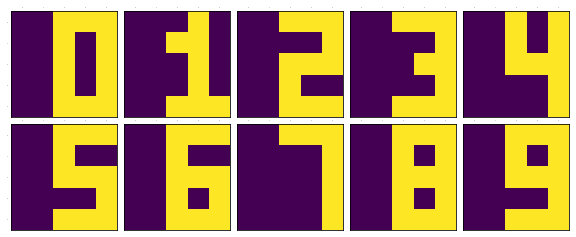
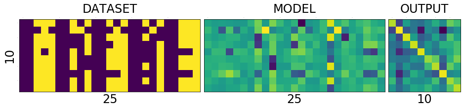
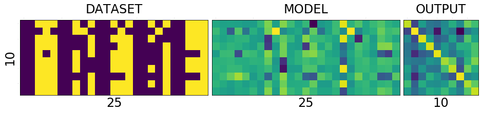
Lets take a look into how the dataset looks like

import matplotlib.pyplot as plt
from mpl_toolkits.axes_grid1 import ImageGrid
from PIL import Image
import pprint
import numpy

num_of_samples = 5

fig = plt.figure(1,(8., 8.))
grid = ImageGrid(fig, 111,
                 nrows_ncols=(num_of_samples, num_of_samples),
                 axes_pad=0.1)

output = numpy.zeros(num_of_samples ** 2)
for i, (data, target) in enumerate(test_loader):
    if i < 1: #dirty trick to take just one sample
        for j in range(num_of_samples ** 2):
            grid[j].matshow(Image.fromarray(data[j][0].numpy()))
            output[j] = target[j]
    else:
        break


output = output.reshape(num_of_samples, num_of_sample)
plt.show()
[[ 6.  9.  9.  5.  4.]
 [ 3.  6.  5.  0.  1.]
 [ 8.  1.  3.  6.  2.]
 [ 9.  4.  8.  8.  6.]
 [ 0.  6.  4.  2.  3.]]
/images/mnist_study_in_pytorch/output_12_0.png

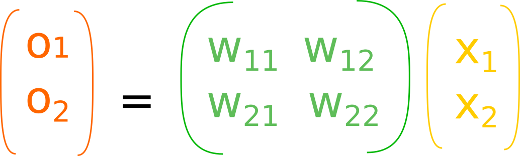
You can see that the image of number <> is associated with number <>. It is a list of (image of number, number). As usual we are gonna feed the neural network with image from the left and its label from the right. We will train a set of feedforward networks in increasing order of complexity. What I mean by complexity is the number of neurons and number of layers.

class Model0(nn.Module):
    def __init__(self):
        super(Model0, self).__init__()
        self.output_layer = nn.Linear(28*28, 10)

    def forward(self, x):
        x = self.output_layer(x)
        return F.log_softmax(x)

class Model1(nn.Module):
    def __init__(self):
        super(Model1, self).__init__()
        self.input_layer = nn.Linear(28*28, 5)
        self.output_layer = nn.Linear(5, 10)

    def forward(self, x):
        x = self.input_layer(x)
        x = self.output_layer(x)
        return F.log_softmax(x)

class Model2(nn.Module):
    def __init__(self):
        super(Model2, self).__init__()
        self.input_layer = nn.Linear(28*28, 6)
        self.output_layer = nn.Linear(6, 10)

    def forward(self, x):
        x = self.input_layer(x)
        x = self.output_layer(x)
        return F.log_softmax(x)

class Model3(nn.Module):
    def __init__(self):
        super(Model3, self).__init__()
        self.input_layer = nn.Linear(28*28, 7)
        self.output_layer = nn.Linear(7, 10)

    def forward(self, x):
        x = self.input_layer(x)
        x = self.output_layer(x)
        return F.log_softmax(x)

class Model4(nn.Module):
    def __init__(self):
        super(Model4, self).__init__()
        self.input_layer = nn.Linear(28*28, 8)
        self.output_layer = nn.Linear(8, 10)

    def forward(self, x):
        x = self.input_layer(x)
        x = self.output_layer(x)
        return F.log_softmax(x)

class Model5(nn.Module):
    def __init__(self):
        super(Model5, self).__init__()
        self.input_layer = nn.Linear(28*28, 9)
        self.output_layer = nn.Linear(9, 10)

    def forward(self, x):
        x = self.input_layer(x)
        x = self.output_layer(x)
        return F.log_softmax(x)

class Model6(nn.Module):
    def __init__(self):
        super(Model6, self).__init__()
        self.input_layer = nn.Linear(28*28, 10)
        self.output_layer = nn.Linear(10, 10)

    def forward(self, x):
        x = self.input_layer(x)
        x = self.output_layer(x)
        return F.log_softmax(x)

class Model7(nn.Module):
    def __init__(self):
        super(Model7, self).__init__()
        self.input_layer = nn.Linear(28*28, 100)
        self.output_layer = nn.Linear(100, 10)

    def forward(self, x):
        x = self.input_layer(x)
        x = self.output_layer(x)
        return F.log_softmax(x)

class Model8(nn.Module):
    def __init__(self):
        super(Model8, self).__init__()
        self.input_layer = nn.Linear(28*28, 100)
        self.hidden_layer = nn.Linear(100, 100)
        self.output_layer = nn.Linear(100, 10)

    def forward(self, x):
        x = self.input_layer(x)
        x = self.hidden_layer(x)
        x = self.output_layer(x)
        return F.log_softmax(x)

class Model9(nn.Module):
    def __init__(self):
        super(Model9, self).__init__()
        self.input_layer = nn.Linear(28*28, 100)
        self.hidden_layer = nn.Linear(100, 100)
        self.hidden_layer1 = nn.Linear(100, 100)
        self.output_layer = nn.Linear(100, 10)

    def forward(self, x):
        x = self.input_layer(x)
        x = self.hidden_layer(x)
        x = self.hidden_layer1(x)
        x = self.output_layer(x)
        return F.log_softmax(x)

class Model10(nn.Module):
    def __init__(self):
        super(Model10, self).__init__()
        self.input_layer = nn.Linear(28*28, 100)
        self.hidden_layer = nn.Linear(100, 100)
        self.hidden_layer1 = nn.Linear(100, 100)
        self.hidden_layer2 = nn.Linear(100, 100)
        self.output_layer = nn.Linear(100, 10)

    def forward(self, x):
        x = self.input_layer(x)
        x = self.hidden_layer(x)
        x = self.hidden_layer1(x)
        x = self.hidden_layer2(x)
        x = self.output_layer(x)
        return F.log_softmax(x)

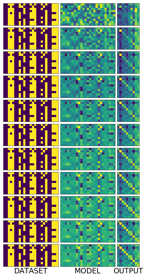
Lets create the model instances. If you have GPU this is how you can make use of it, by calling .cuda() on models and tensors

models = Model0(), Model1(), Model2(), Model3(), Model4(), Model5(), Model6(), Model7(), Model8(), Model9(), Model10()
if args.cuda:
    for model in models:
        model.cuda()
def train(epoch, model, print_every=100):
    optimizer = optim.SGD(model.parameters(), lr=args.lr, momentum=args.momentum)
    for i in range(epoch):
        model.train()
        for batch_idx, (data, target) in enumerate(train_loader):
            if args.cuda:
                data, target = data.cuda(), target.cuda()
            data = data.view(args.batch_size , -1)
            data, target = Variable(data), Variable(target)
            optimizer.zero_grad()
            output = model(data)

            loss = F.nll_loss(output, target)
            loss.backward()
            optimizer.step()

        if i % print_every == 0:
            print('Train Epoch: {} [{}/{} ({:.0f}%)]\tLoss: {:.6f}'.format(
                    i, batch_idx * len(data), len(train_loader.dataset),
                    100. * batch_idx / len(train_loader), loss.data[0]))

This is where the actual training starts. It will take a while, so I just trained them for 100 times on entire training dataset.

for model in models:
    train(100, model)
Train Epoch: 0 [59988/60000 (100%)]        Loss: 0.061506
.
.
.
.
Train Epoch: 98 [59988/60000 (100%)]       Loss: 0.018422
Train Epoch: 99 [59988/60000 (100%)]       Loss: 0.336890

Saving the model weights into a file, this should be in the above snippet or inside the training function for saving models every epoch.Lets just keep this simple

for i, model in enumerate(models):
    torch.save(model.state_dict(), 'mnist_mlp_multiple_model{}.pth'.format(i))

For the sake of completeness, this is how you load the saved models

models = Model0(), Model1(), Model2(), Model3(), Model4(), Model5(), Model6(), Model7(), Model8(), Model9(), Model10()
if args.cuda:
    for model in models:
        model.cuda()

for i, model in enumerate(models):
    model.load_state_dict(torch.load('mnist_mlp_multiple_model{}.pth'.format(i)))

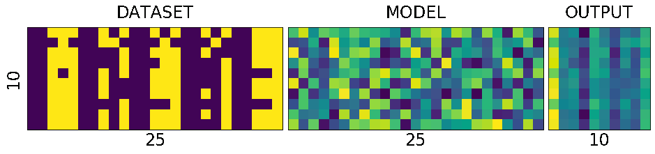
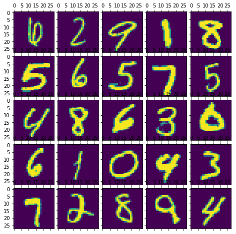
Before we run the model over the test dataset, let take a peek into how one of the model performs

%matplotlib inline
import matplotlib.pyplot as plt
from mpl_toolkits.axes_grid1 import ImageGrid
from PIL import Image
import pprint
import numpy

fig = plt.figure(1,(8., 8.))
grid = ImageGrid(fig, 111,  # similar to subplot(111)
                 nrows_ncols=(3, 3),  # creates 2x2 grid of axes
                 axes_pad=0.1,  # pad between axes in inch.
                 )

output = numpy.zeros(9)
for i, (data, target) in enumerate(test_loader):
    if i < 1: #dirty trick

        data1 = data.cuda()
        data1 = data1.view(data.size()[0], -1)
        out = models[9](Variable(data1))

        for j in range(9):
            grid[j].matshow(Image.fromarray(data[j][0].numpy()))
            output[j] = out.data.max(1)[1][j].cpu().numpy()[0]

    else:
        break

output = output.reshape(3,3)
print(output)
plt.show()
[[ 6.  2.  9.  1.  8.]
 [ 5.  6.  5.  7.  5.]
 [ 4.  8.  6.  3.  0.]
 [ 6.  1.  0.  9.  3.]
 [ 7.  2.  8.  4.  4.]]
/images/mnist_study_in_pytorch/output_12_0.png

As you can see, the results are not so bad.Lets test all our models.

def test(model):
    model.eval()
    test_loss = 0
    correct = 0
    for data, target in test_loader:
        if args.cuda:
            data, target = data.cuda(), target.cuda()

        data = data.view(data.size()[0], -1)
        data, target = Variable(data, volatile=True), Variable(target)
        output = model(data)
        test_loss += F.nll_loss(output, target).data[0]
        pred = output.data.max(1)[1] # get the index of the max log-probability
        correct += pred.eq(target.data).cpu().sum()

    test_loss = test_loss
    test_loss /= len(test_loader) # loss function already averages over batch size
    print('\nTest set: Average loss: {:.4f}, Accuracy: {}/{} ({:.0f}%)\n'.format(
        test_loss, correct, len(test_loader.dataset),
        100. * correct / len(test_loader.dataset)))

    return 100. * correct / len(test_loader.dataset)
%matplotlib inline
import matplotlib.pyplot as plt
from mpl_toolkits.axes_grid1 import ImageGrid
from PIL import Image
import pprint
import numpy


accuracy = []
for model in models:
    accuracy.append(test_tuts(model))

pprint.pprint(accuracy)
Test set: Average loss: 0.2764, Accuracy: 9250/10000 (92%)
Test set: Average loss: 0.3591, Accuracy: 9010/10000 (90%)
Test set: Average loss: 0.3204, Accuracy: 9121/10000 (91%)
Test set: Average loss: 0.2954, Accuracy: 9189/10000 (92%)
Test set: Average loss: 0.2767, Accuracy: 9237/10000 (92%)
Test set: Average loss: 0.2699, Accuracy: 9267/10000 (93%)
Test set: Average loss: 0.2700, Accuracy: 9251/10000 (93%)
Test set: Average loss: 0.2690, Accuracy: 9244/10000 (92%)
Test set: Average loss: 0.2755, Accuracy: 9240/10000 (92%)
Test set: Average loss: 0.2745, Accuracy: 9253/10000 (93%)
Test set: Average loss: 0.2789, Accuracy: 9232/10000 (92%)

[92.5, 90.1, 91.21, 91.89, 92.37, 92.67, 92.51, 92.44, 92.4, 92.53, 92.32]
plt.plot(range(len(accuracy)), accuracy, linewidth=1.0)
plt.axis([0, 10, 0, 100])
plt.show()

plt.plot(range(len(accuracy)), accuracy, linewidth=1.0)
plt.axis([0, 10, 90, 93])
plt.show()
/images/mnist_study_in_pytorch/output_11_0.png/images/mnist_study_in_pytorch/output_11_1.png

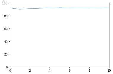
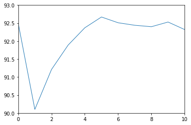
The right image is a little zoomed in version of the left one. Little dissappointing, isn't it? The more complex models doesn't seem to perform as we would expect. So we can understand that the performance is not proportional to number of layers in neural network. It is in how they interact with each other.

PyTorch Primer

This is post is inspired by Numpy Primer <http://suriyadeepan.github.io/2016-06-26-numpy-primer/>

Lets create some matrices

 import torch

 x = torch.zeros(3, 3)
 print(x)

 0  0  0
 0  0  0
 0  0  0
[torch.FloatTensor of size 3x3]


 x = torch.ones(3, 3)
 print(x)

 1  1  1
 1  1  1
 1  1  1
[torch.FloatTensor of size 3x3]


 x = torch.randn(3, 3)
 print(x)

-0.0008 -0.6619 -0.6790
 0.9104 -0.1249 -0.4044
-1.0516 -0.4031  0.9166
[torch.FloatTensor of size 3x3]

I think now we can understand what the parameters to the above functions mean - the shape of the tensor. Take a look at non square matrices below

 x = torch.zeros(2,4)
 print(x)

 0  0  0  0
 0  0  0  0
[torch.FloatTensor of size 2x4]


 x = torch.zeros(4,3)
 print(x)

 0  0  0
 0  0  0
 0  0  0
 0  0  0
[torch.FloatTensor of size 4x3]

How about a multidimensional vector - a tensor. Actually tensor is a general term for n-dimensional arrays like in numpy. If you were keen observant, you'd have notices by now that the output of every print(x) end with torch.FloatTensor. This term became famous with the deep learning storm.

 x = torch.zeros(2, 3, 2, 2, 3)
 print(x)

(0 ,0 ,0 ,.,.) =
  0  0  0
  0  0  0

(0 ,0 ,1 ,.,.) =
  0  0  0
  0  0  0

(0 ,1 ,0 ,.,.) =
  0  0  0
  0  0  0

(0 ,1 ,1 ,.,.) =
  0  0  0
  0  0  0

(0 ,2 ,0 ,.,.) =
  0  0  0
  0  0  0

(0 ,2 ,1 ,.,.) =
  0  0  0
  0  0  0

(1 ,0 ,0 ,.,.) =
  0  0  0
  0  0  0

(1 ,0 ,1 ,.,.) =
  0  0  0
  0  0  0

(1 ,1 ,0 ,.,.) =
  0  0  0
  0  0  0

(1 ,1 ,1 ,.,.) =
  0  0  0
  0  0  0

(1 ,2 ,0 ,.,.) =
  0  0  0
  0  0  0

(1 ,2 ,1 ,.,.) =
  0  0  0
  0  0  0
[torch.FloatTensor of size 2x3x2x2x3]

Pause for a moment and take a long look into how the tensor is printed. And then proceed to look for more matrices below. The identity matrix - matrix is the keyword.

# The identity matrix - max upto two dimensions
x = torch.eye(3)
print(x)

 1  0  0
 0  1  0
 0  0  1
[torch.FloatTensor of size 3x3]


x = torch.eye(3,4)
print(x)

 1  0  0  0
 0  1  0  0
 0  0  1  0
[torch.FloatTensor of size 3x4]

Alright I get it. Just ones and zeros are boring. Want some more numbers? torch.linspace(start, end, count) creates a list of numbers starting with start to end at the interval of (end - start)/(count - 1)

 x = torch.linspace(1, 6, 10)
 print(x)

 1.0000
 1.5556
 2.1111
 2.6667
 3.2222
 3.7778
 4.3333
 4.8889
 5.4444
 6.0000
[torch.FloatTensor of size 10]

torch.logspace() is similar to torch.linspace() but in logarthmic steps.

 x = torch.logspace(.1, 1, 5)
 print(x)

  1.2589
  2.1135
  3.5481
  5.9566
 10.0000
[torch.FloatTensor of size 5]

Arithmetics

So what we created bunch of numbers. What is the use? Lets do some arithmetic

Elementwise addition

 x = torch.ones(3)
 print(x)

 1
 1
 1
[torch.FloatTensor of size 3]


 y = x + 2
 print(y)

 3
 3
 3
[torch.FloatTensor of size 3]

Elementwise multiplication

 x = torch.range(1, 10)
 print(x)

  1
  2
  3
  4
  5
  6
  7
  8
  9
 10
[torch.FloatTensor of size 10]

 y = x * 2
 print(y)

  2
  4
  6
  8
 10
 12
 14
 16
 18
 20
[torch.FloatTensor of size 10]

Iterating over the elements and multiplying them by some number

for i in range(10):
    y[i] = x[i] * i

print(y)

  0
  2
  6
 12
 20
 30
 42
 56
 72
 90
[torch.FloatTensor of size 10]

So yes we can multiply the tensors by ordinary numbers, there is no need for 'i' to be a tensor, lets take a larger tensors, and assign its values by hand. So far we have been using the numbers generated by function like ones(), zeros() and rand(). In most cases we need our favoruite numbers. How to do this? torch.Tensor() to the rescue.

x = torch.Tensor([1,3,5,6,78,3,67])
print(x)

  1
  3
  5
  6
 78
  3
 67
[torch.FloatTensor of size 7]

x = torch.Tensor([range(0, 10, 2), range(10, 20, 2), range(20, 25)])
print(x)

  0   2   4   6   8
 10  12  14  16  18
 20  21  22  23  24
[torch.FloatTensor of size 3x5]

As we can see, the torch.Tensor() takes any iterable or iterables of iterable and makes a tensor out of it

Broadcasting Adding a scalar to a tensor or multiplying a tensor by a scalar is essentially same as adding or multiplying the tensor by another tensor with shape same as the original tensor, with all its elements being the scalar. Too many words.

x = torch.linspace(1, 10, 10)
print(x)

  1
  2
  3
  4
  5
  6
  7
  8
  9
 10
[torch.FloatTensor of size 10]


w = torch.Tensor([2])
print(w)

 2
[torch.FloatTensor of size 1]


# broadcasting  https://discuss.pytorch.org/t/broadcasting-or-alternative-solutions/120
y = w.expand_as(x) * x
print(y)

  2
  4
  6
  8
 10
 12
 14
 16
 18
 20
[torch.FloatTensor of size 10]


w = torch.Tensor([2, 3])
print(w)

 2
 3
[torch.FloatTensor of size 2]

y = w.expand_as(x) * x        #Dont' work
Traceback (most recent call last):
  File "<stdin>", line 1, in <module>
  File "/home/paarulakan/environments/python/pytorch-py35/lib/python3.5/site-packages/torch/tensor.py", line 274, in expand_as
    return self.expand(tensor.size())
  File "/home/paarulakan/environments/python/pytorch-py35/lib/python3.5/site-packages/torch/tensor.py", line 261, in expand
    raise ValueError('incorrect size: only supporting singleton expansion (size=1)')
ValueError: incorrect size: only supporting singleton expansion (size=1)

Note that the expand_as() works only for singletons

Reshaping Tensors

view() takes list of number and reshapes the tensor as per the arguments.

The constrain is for view(a, b, c,....n) a x b x c x ... x n should be equal to the size of the given tensor. If you give '-1' as the last argument to view() it will calculate the last dimension by itself.

x = x.view(2, 5)
print(x)

  1  2  3  4  5
  6  7  8  9  10
[torch.FloatTensor of size 2x5]

# making matrices by hand is hard right?
x  = torch.range(1, 16)
x_ = x.view(2, 8)
print(x_)

    1     2     3     4     5     6     7     8
    9    10    11    12    13    14    15    16
[torch.FloatTensor of size 2x8]


x_ = x.view(2, 2, 4)
print(x_)

(0 ,.,.) =
   1   2   3   4
   5   6   7   8

(1 ,.,.) =
   9  10  11  12
  13  14  15  16
[torch.FloatTensor of size 2x2x4]


x_ = x.view(2, 2, 2, -1)
print(x_)

(0 ,0 ,.,.) =
   1   2
   3   4

(0 ,1 ,.,.) =
   5   6
   7   8

(1 ,0 ,.,.) =
   9  10
  11  12

(1 ,1 ,.,.) =
  13  14
  15  16
[torch.FloatTensor of size 2x2x2x2]


x[5] = -1 * x[5]
print(x_)

(0 ,0 ,.,.) =
   1   2
   3   4

(0 ,1 ,.,.) =
   5  -6
   7   8

(1 ,0 ,.,.) =
   9  10
  11  12

(1 ,1 ,.,.) =
  13  14
  15  16
[torch.FloatTensor of size 2x2x2x2]

Notice that change in value of an element in x reflects in x_. It is because view() does exactly what is says it will do. It creates a view of the tensor, the underlying storage is same for x and x_

Statistics

x  = torch.range(1, 16)
x_ = x.view(4,4)
print(x_)

  1   2   3   4
  5   6   7   8
  9  10  11  12
 13  14  15  16
[torch.FloatTensor of size 4x4]

print(x_.sum(dim = 0))

 28  32  36  40
[torch.FloatTensor of size 1x4]

print(x_.sum(dim = 1))

 10
 26
 42
 58
[torch.FloatTensor of size 4x1]

x_ = x.view(2,2,4)
print(x_)

(0 ,.,.) =
   1   2   3   4
   5   6   7   8

(1 ,.,.) =
   9  10  11  12
  13  14  15  16
[torch.FloatTensor of size 2x2x4]

print(x_.sum(dim = 0))

(0 ,.,.) =
  10  12  14  16
  18  20  22  24
[torch.FloatTensor of size 1x2x4]

print(x_.sum(dim = 1))

(0 ,.,.) =
   6   8  10  12

(1 ,.,.) =
  22  24  26  28
[torch.FloatTensor of size 2x1x4]

print(x_.sum(dim = 2))

(0 ,.,.) =
  10
  26

(1 ,.,.) =
  42
  58
[torch.FloatTensor of size 2x2x1]

Matrix Multiplication

mm() is name. See how it is different from normal elementwise multiplication, like we used to do in linear algebra class?

#lets do some matrix multiplications
w = torch.Tensor([[10, 20],
                  [30, 40]])

x = torch.Tensor([[1,2],
                  [3,4]])

print(w.mm(x))

  70  100
 150  220
[torch.FloatTensor of size 2x2]

w = torch.Tensor([[10, 20],
                  [30, 40],
                  [50, 60]])

x = torch.Tensor([[1,2,5],
                  [3,4,6]])
print(w.mm(x))

  70  100  170
 150  220  390
 230  340  610
[torch.FloatTensor of size 3x3]

Indexing and slicing

#Indexing and slicing
x = torch.range(1, 64)
print(x)

  1
  2
  3
  4
  5
  .
  .
  .
 61
 62
 63
 64

[torch.FloatTensor of size 64]


x_ = x.view(4,4,4)
print(x_)

(0 ,.,.) =
   1   2   3   4
   5   6   7   8
   9  10  11  12
  13  14  15  16

(1 ,.,.) =
  17  18  19  20
  21  22  23  24
  25  26  27  28
  29  30  31  32

(2 ,.,.) =
  33  34  35  36
  37  38  39  40
  41  42  43  44
  45  46  47  48

(3 ,.,.) =
  49  50  51  52
  53  54  55  56
  57  58  59  60
  61  62  63  64
[torch.FloatTensor of size 4x4x4]

print(x_[1, 1, :])

 21
 22
 23
 24
[torch.FloatTensor of size 4]

Masking

#the expression 'x_ % 4 == 0' creates a mask
print(x_ % 4 == 0)

(0 ,.,.) =
  0  0  0  1
  0  0  0  1
  0  0  0  1
  0  0  0  1

(1 ,.,.) =
  0  0  0  1
  0  0  0  1
  0  0  0  1
  0  0  0  1

(2 ,.,.) =
  0  0  0  1
  0  0  0  1
  0  0  0  1
  0  0  0  1

(3 ,.,.) =
  0  0  0  1
  0  0  0  1
  0  0  0  1
  0  0  0  1
[torch.ByteTensor of size 4x4x4]

# Use the mask to extract just those elements

x_[0][(x_%4 == 0)[0]]

  4
  8
 12
 16
[torch.FloatTensor of size 4]


#more grander masking example

x = torch.range(1, 64)
print(x)

  1
  2
  3
  4
  5
  .
  .
  .
 61
 62
 63
 64

[torch.FloatTensor of size 64]

x_ = x.view(8,8)
print(x_)

    1     2     3     4     5     6     7     8
    9    10    11    12    13    14    15    16
   17    18    19    20    21    22    23    24
   25    26    27    28    29    30    31    32
   33    34    35    36    37    38    39    40
   41    42    43    44    45    46    47    48
   49    50    51    52    53    54    55    56
   57    58    59    60    61    62    63    64
[torch.FloatTensor of size 8x8]

x_ind = torch.eye(8).byte()
print(x_ind)

    1     0     0     0     0     0     0     0
    0     1     0     0     0     0     0     0
    0     0     1     0     0     0     0     0
    0     0     0     1     0     0     0     0
    0     0     0     0     1     0     0     0
    0     0     0     0     0     1     0     0
    0     0     0     0     0     0     1     0
    0     0     0     0     0     0     0     1
[torch.ByteTensor of size 8x8]

print(x[x_ind])

  1
 10
 19
 28
 37
 46
 55
 64
[torch.FloatTensor of size 8]

Please leave your comments below.

VanangamudiMNIST

WORK IN PROGRESS

The problem I designed for this post came to me when I was trying to explain neural network to my friend who is just getting started on it. The hello world of deep learning is MNIST, but the size of the MNIST images is 28x28 which is too large to help us understand the ideas in terms of observable concrete computations and visualizations. So here you go.

Note: It is not my intention for you to read the code. I advice against it. I include the code in the post for the reason that, if anyone interested in trying it out in their desktop or laptop, they should be able to. Please don't read the code, focus on the concepts and computations :)

import torch
from torch.autograd import Variable

DATASET

Dataset is a collection of data. What is in a dataset and why we need it?

dataset = [] #list of tuples (image, label)

zer = torch.Tensor([[0, 0, 1, 1, 1],
                    [0, 0, 1, 0, 1],
                    [0, 0, 1, 0, 1],
                    [0, 0, 1, 0, 1],
                    [0, 0, 1, 1, 1],
                   ])

one = torch.Tensor([[0, 0, 0, 1, 0],
                    [0, 0, 1, 1, 0],
                    [0, 0, 0, 1, 0],
                    [0, 0, 0, 1, 0],
                    [0, 0, 1, 1, 1],
                   ])

two = torch.Tensor([[0, 0, 1, 1, 1],
                    [0, 0, 0, 0, 1],
                    [0, 0, 1, 1, 1],
                    [0, 0, 1, 0, 0],
                    [0, 0, 1, 1, 1],
                   ])

thr = torch.Tensor([[0, 0, 1, 1, 1],
                    [0, 0, 0, 0, 1],
                    [0, 0, 0, 1, 1],
                    [0, 0, 0, 0, 1],
                    [0, 0, 1, 1, 1],
                   ])

fou = torch.Tensor([[0, 0, 1, 0, 1],
                    [0, 0, 1, 0, 1],
                    [0, 0, 1, 1, 1],
                    [0, 0, 0, 0, 1],
                    [0, 0, 0, 0, 1],
                   ])

fiv = torch.Tensor([[0, 0, 1, 1, 1],
                    [0, 0, 1, 0, 0],
                    [0, 0, 1, 1, 1],
                    [0, 0, 0, 0, 1],
                    [0, 0, 1, 1, 1],
                   ])

six = torch.Tensor([[0, 0, 1, 1, 1],
                    [0, 0, 1, 0, 0],
                    [0, 0, 1, 1, 1],
                    [0, 0, 1, 0, 1],
                    [0, 0, 1, 1, 1],
                   ])

sev = torch.Tensor([[0, 0, 1, 1, 1],
                    [0, 0, 0, 0, 1],
                    [0, 0, 0, 0, 1],
                    [0, 0, 0, 0, 1],
                    [0, 0, 0, 0, 1],
                   ])

eig = torch.Tensor([[0, 0, 1, 1, 1],
                    [0, 0, 1, 0, 1],
                    [0, 0, 1, 1, 1],
                    [0, 0, 1, 0, 1],
                    [0, 0, 1, 1, 1],
                   ])

nin = torch.Tensor([[0, 0, 1, 1, 1],
                    [0, 0, 1, 0, 1],
                    [0, 0, 1, 1, 1],
                    [0, 0, 0, 0, 1],
                    [0, 0, 1, 1, 1],
                   ])

dataset.append((zer, torch.Tensor([0])))
dataset.append((one, torch.Tensor([1])))
dataset.append((two, torch.Tensor([2])))
dataset.append((thr, torch.Tensor([3])))
dataset.append((fou, torch.Tensor([4])))
dataset.append((fiv, torch.Tensor([5])))
dataset.append((six, torch.Tensor([6])))
dataset.append((sev, torch.Tensor([7])))
dataset.append((eig, torch.Tensor([8])))
dataset.append((nin, torch.Tensor([9])))

Take a look into how the data looks like

%matplotlib inline
import matplotlib.pyplot as plt
from mpl_toolkits.axes_grid1 import ImageGrid
from PIL import Image

fig = plt.figure(1,(10., 50.))
grid = ImageGrid(fig, 111,
                 nrows_ncols=(2 , 5),
                 axes_pad=0.1)

for i, (data, target) in enumerate(dataset):
    grid[i].matshow(Image.fromarray(data.numpy()))
    grid[i].tick_params(axis='both', which='both', length=0, labelsize=0)
plt.show()
/images/vanangamudimnist/output_5_0.png

We have a set of 10 images of numbers 0..9. We want to make a neural network to predict what is the number on the image.

MODEL

Model is the term we use to refer to the network. Our model is a simple 25x10 matrix. Don't get startled by the class and the imports. It just does matrix multiplication. For now assume *model()* is a function which will take in a matrix of size (AxB) as input and mutiply it with the network weight matrix of size (BxC), to produce another matrix as output of size (AxC).

from torch import nn
import torch.nn.functional as F
import torch.optim as optim

class Model(nn.Module):
    def __init__(self):
        super(Model, self).__init__()
        self.output_layer = nn.Linear(5*5, 10, bias=False)

    def forward(self, x):
        x = self.output_layer(x)
        return F.log_softmax(x)
model = Model()
optimizer = optim.SGD(model.parameters(), lr=1, momentum=0.1)

DATASET - MODEL - OUTPUT

To understand the network and its training process, it is helpful to see the holy trinity INPUT-MODEL-OUTPUT

fig = plt.figure(1, (16., 16.))
grid = ImageGrid(fig, 111,
                     nrows_ncols=(1, 3),
                     axes_pad=0.1)


data = [data.view(-1) for data, target in dataset]
data = torch.stack(data)

target = [target.view(-1) for data, target in dataset]
target = torch.stack(target).squeeze()
grid[0].matshow(Image.fromarray(data.numpy()))
grid[0].set_title('DATASET', fontsize=24)
grid[0].set_ylabel('10', fontsize=24)
grid[0].set_xlabel('25', fontsize=24)
grid[0].tick_params(axis='both', which='both', length=0, labelsize=0)

grid[1].matshow(Image.fromarray(model.output_layer.weight.data.numpy()))
grid[1].set_title('MODEL', fontsize=24)
grid[1].set_xlabel('25', fontsize=24)
grid[1].tick_params(axis='both', which='both', length=0, labelsize=0)


output = model(Variable(data))
grid[2].matshow(Image.fromarray(output.data.numpy()))
grid[2].set_title('OUTPUT', fontsize=24)
grid[2].set_xlabel('10', fontsize=24)
grid[2].tick_params(axis='both', which='both', length=0, labelsize=0)

plt.show()
/images/vanangamudimnist/output_11_0.png

Lets try to understand what is in the picture above.

The first one is the collection of all the data that we have. The second one is the matrix of weights connecting the input of 25 input neurons to 10 output neurons. And the last one we will get to it little later.

What is special about 25 and 10 here?

Nothing. Our dataset is a set of images of numbers each having a size of 5x5 ==> 25. And we have how many different numbers a hand? 0,1,2...9 ==> 10 numbers or 10 different classes of output(this will become clear in the next post)

What is that weird picture on the left, having weird

  • zero in the top-left,
  • and three on the bottom-right
  • and some messed up fours and eights in the middle.

Let get to it. Look the picture below.

fig = plt.figure(1,(12., 12.))
grid = ImageGrid(fig, 111,
                 nrows_ncols=(2 , 5),
                 axes_pad=0.1)

for i, (d, t) in enumerate(dataset):
    grid[i].matshow(Image.fromarray(d.numpy()))
    grid[i].tick_params(axis='both', which='both', length=0, labelsize=0)

plt.show()

fig = plt.figure(1, (100., 10.))
grid = ImageGrid(fig, 111,
                     nrows_ncols=(len(dataset), 1),
                     axes_pad=0.1)


data = [data.view(1, -1) for data, target in dataset]

for i, d in enumerate(data):
    grid[i].matshow(Image.fromarray(d.numpy()))
    grid[i].set_ylabel('{}'.format(i), fontsize=36)
    grid[i].tick_params(axis='both', which='both', length=0, labelsize=0)
/images/vanangamudimnist/output_13_0.png/images/vanangamudimnist/output_13_1.png

Voila!! We have just arranged the image matrix into a vector. TODO why?

This is important to remember, a simple neural network looks at the input and try to figure out which class does this input belong to

In our case inputs are the images of numbers, and outputs are how similar are the classes to the input. The output neuron with highest value is closer(very similar) to the input and the output neuron with least value is very NOT similar to the input. The inputs are real valued - it can take any numerical value but the output is discrete, a whole number corresponding to index of the neuron with largest numerical value. Also note that output of the network does not mean output of neurons.

For example after training, if we feed the image of number 3, the output neurons corresponding to 3, 8, 9 and probably 7 will have larger values and the output neurons corresponding to 1 and 6 will have the least value. Don't worry if you don't understand why, it will become clearer as we go on.

How many correct predictions without any training

Too much theory, lets get our hands dirty. Let see how many numbers did our model predicted correctly.

# Remember that output = model(Variable(data))
pred = output.data.max(1)[1].squeeze()
print(pred.size(), target.size())
correct = pred.eq(target.long()).sum()
print('correct: {}/{}'.format(correct, len(dataset)))
torch.Size([10]) torch.Size([10])
correct: 1/10

(N)ONE out of TEN

That is right it predicted none out of ten. We feeded our network with all of our data and asked it to figure what is the number that is in the image. Remember what we learned earlier about output neurons. The neural network tell us which number is present in the image by lighting up that corresponding neuron. Lets say if gave 6, the network will light up the 6th neuron will be the brightest, i.e the 6th neurons value will be the highest compared to all other neurons.

But our network above lit up wrong bulbs, for all the output. None out of ten. But why? Isn't neural network are supposed to smarter? Well yes and no. That is the difference between traditional image processing algorithms and neural networks.

Wait, let me tell you a story, that I heard. During the second world war, there were skilled flight spotter. Their job was to spot and report if any air craft was approaching. As the war got intense, there was need for more spotters and there were lot of volunteers even from schools and colleges but there was very little time to train them. So the skilled spotters, listed out a set of things to look for in the enemy flights and asked the new volunteers to memorize them as part of the training. But the volunteers never got good at spotting. Ooosh, we will continue the story later, lets get back to the point.

In classical image processing systems, we humans think, think and think and think a lot more and come up a set of rules or instructions, just like those skilled spotters. We give those instructions to the system, to make it understand how to process the images to extract information(called features - things to look for in the enemy flight) from them, and then use that information to make further decisions, such predicting what number is in the image. We feed that system with knowledge first before asking it to do anything for us.

But did we feed any knowledge to network? We just told it the input size is 25 and output size is 10. How can you expect someone to guess what is in your hand, by just telling them its size. That is rude of you. Shame on you. Okay okay. How do we make the system more knowledgable about the input? Training. The holy grail of deep learning.

What is training?

We know that the knowledge of the neural network is in the weights of the connections - represented as matrix above. We also know that by multiplying this matrix by an input image vector we will get an output which is a set of scores that describes, how similar the input is to the output neurons.

Imagine giving random values to the weights and feed the network with our data and see whether it predicts all our numbers correctly. If it did, fine and dandy, but if not give random values to the weights again and repeat the process until our network predicts all the numbers correctly. That is training in most simple form.

But think about how long will it take to find such random magical values for every weight in the network to make it work as expected. We don't know that for sure. right? You wanna continue the story. don't you? Alright.

The skilled people tried as much as they can to identify the distinguishing features of the home and enemy air crafts and tried to make the volunteers understand them. It never worked. Then they changes the strategy. They put them on the job and made them learn themselves. i.e every skilled spotter will have ten volunteers and whenever an aircraft is seen, the volunteers will shout the kind of the plane, say 'german'. Then the skilled one, will reveal the correct answer. This technique was extrememly sucessful, a spotter sent in an emergency message not only identifying it as a German aircraft, but also the correct make and model..more

Hey, why don't we try the same with our network? Lets feed the images into it and shout the answer into its tiny little output neurons so that it can update its weights by itself. Now I know you're asking how can we expect, a dumb network which cannot even predict a number in an image to train itself? Well that is where it gets interesting. We can't. Backpropgation to the rescue. It is the algorithm to update the weights of the network on our behalf.

It looks at how difference between output of network and desired output, changes with respect to the weights, and then it modifies the weights based on it. [2]

So now you understand why it predicted none out of ten correctly.

import sys
def test_and_print(model, dataset, title='', plot=True):

    data = [data.view(-1) for data, target in dataset]
    data = torch.stack(data).squeeze()

    target = [target.view(-1) for data, target in dataset]
    target = torch.stack(target).squeeze()
    output = model(Variable(data))

    loss = F.nll_loss(output, Variable(target.long()))

    dataset_img = Image.fromarray(data.numpy())
    model_img   = Image.fromarray(model.output_layer.weight.data.numpy())
    output_img  = Image.fromarray(output.data.numpy())

    pred = output.data.max(1)[1]
    correct = pred.eq(target.long()).sum()

    print('correct: {}/{}, loss:{}'.format(correct, len(dataset), loss.data[0]))
    sys.stdout.flush()

    if plot:
        fig = plt.figure(1,(16., 16.))
        grid = ImageGrid(fig, 111,
                         nrows_ncols=(1 , 3),
                         axes_pad=0.1)

        grid[0].matshow(dataset_img)
        grid[0].set_title('DATASET', fontsize=24)
        grid[0].tick_params(axis='both', which='both', length=0, labelsize=0)
        grid[0].set_ylabel('10', fontsize=24)
        grid[0].set_xlabel('25', fontsize=24)

        grid[1].matshow(model_img)
        grid[1].set_title('MODEL', fontsize=24)
        grid[1].tick_params(axis='both', which='both', length=0, labelsize=0)
        grid[1].set_xlabel('25', fontsize=24)

        grid[2].matshow(output_img)
        grid[2].set_title('OUTPUT', fontsize=24)
        grid[2].tick_params(axis='both', which='both', length=0, labelsize=0)
        grid[2].set_xlabel('10', fontsize=24)

        plt.show()


    return dataset_img, model_img, output_img

Lets take a closer look at DATASET - MODEL - OUTPUT

and understand what those colors mean.[1]

import numpy
fig = plt.figure(1, (80., 80.))
grid = ImageGrid(fig, 111,
                     nrows_ncols=(1, 3),
                     axes_pad=0.5)


data = [data.view(-1) for data, target in dataset]
data = torch.stack(data)

target = [target.view(-1) for data, target in dataset]
target = torch.stack(target)

grid[0].matshow(Image.fromarray(data.numpy()))
grid[0].set_title('DATASET', fontsize=144)
grid[0].tick_params(axis='both', which='both', length=0, labelsize=0)
grid[0].set_ylabel('10', fontsize=144)
grid[0].set_xlabel('25', fontsize=144)
for (x,y), val in numpy.ndenumerate(data.numpy()):
     grid[0].text(y, x, '{:d}'.format(int(val)), ha='center', va='center', fontsize=24,
            bbox=dict(boxstyle='round', facecolor='white', edgecolor='white'))


grid[1].matshow(Image.fromarray(model.output_layer.weight.data.numpy()))
grid[1].set_title('MODEL', fontsize=144)
grid[1].tick_params(axis='both', which='both', length=0, labelsize=0)
grid[1].set_xlabel('25', fontsize=144)
for (x,y), val in numpy.ndenumerate(model.output_layer.weight.data.numpy()):
     grid[1].text(y, x, '{:0.04f}'.format(val), ha='center', va='center',fontsize=16,
            bbox=dict(boxstyle='round', facecolor='white', edgecolor='white'))

output = model(Variable(data))
grid[2].matshow(Image.fromarray(output.data.numpy()))
grid[2].set_title('OUTPUT', fontsize=144)
grid[2].tick_params(axis='both', which='both', length=0, labelsize=0)
grid[2].set_xlabel('10', fontsize=144)

for (x,y), val in numpy.ndenumerate(output.data.numpy()):
     grid[2].text(y, x, '{:0.04f}'.format(val), ha='center', va='center',fontsize=16,
            bbox=dict(boxstyle='round', facecolor='white', edgecolor='white'))


plt.show()
/images/vanangamudimnist/output_20_0.png

If you zoom in the picture you will see numbers corresponding to the colors - violet means the lowest value, and yellow is the highest values. i.e violet does not mean 0 and yellow does not mean 1 as you might think from the dataset image.

WHAT DOES EACH ROW MEAN?

DATASET

numbers, each row is a number. first one is 0 second one is 1 and so on.

MODEL

weights corresponding to pixels in the image for a number. first row is for 0 and last one is for 9.

OUTPUT

scores of similarity. how similar the input image to all output numbers. First row contains scores of 0, how similar it is to all other numbers first square in the first row is how simlilar 0 is to 0, second square similar it is to 1. Now the scores are not only incorrect but stupid. This will become better and clear as we train the network. Lets take look at the DATASET-MODEL-OUTPUT trinity once again before training

Take look at the following. It shows a single row from the output image. Go on pick the darkest square in the output above. Which row has the darkeset one?, it seems like the row corresponding to number 4, i.e data[4] the least value from that row is -3.0710

print(model(Variable(data[4].view(1, -1))))
Variable containing:
-2.2242 -2.0100 -2.4086 -2.2264 -2.3357 -1.9604 -2.5856 -3.0710 -2.0782 -2.5825
[torch.FloatTensor of size 1x10]

Similarly the brightest yellow is in the row corresonding to number 1 whose value is -1.9198 you can see below. The reason I am stressing about this fact is, this is will influence how we interpret the following images.

print(model(Variable(data[1].view(1, -1))))
Variable containing:
-2.9334 -2.5239 -1.9198 -2.3306 -2.3984 -2.1636 -2.2579 -2.3235 -2.1503 -2.3224
[torch.FloatTensor of size 1x10]
import numpy
def plot_with_values(model, dataset, title=''):
    fig = plt.figure(1, (80., 80.))
    grid = ImageGrid(fig, 111,
                         nrows_ncols=(1, 3),
                         axes_pad=0.5)


    data = [data.view(-1) for data, target in dataset]
    data = torch.stack(data)

    target = [target.view(-1) for data, target in dataset]
    target = torch.stack(target)

    plot_data = [data, model.output_layer.weight.data, model(Variable(data)).data]
    for i, tobeplotted in enumerate(plot_data):
        grid[i].matshow(Image.fromarray(tobeplotted.numpy()))
        grid[i].tick_params(axis='both', which='both', length=0, labelsize=0)
        for (x,y), val in numpy.ndenumerate(tobeplotted.numpy()):
            if i == 0: spec = '{:d}';  val = int(val)
            else: spec = '{:0.2f}'
            grid[i].text(y, x, spec.format(val), ha='center', va='center', fontsize=16,
                bbox=dict(boxstyle='round', facecolor='white', edgecolor='white'))

    grid[0].set_title('DATASET', fontsize=144)
    grid[0].set_ylabel('10', fontsize=144)
    grid[0].set_xlabel('25', fontsize=144)

    grid[1].set_title('MODEL', fontsize=144)
    grid[1].set_xlabel('25', fontsize=144)

    grid[2].set_title('OUTPUT', fontsize=144)
    grid[2].set_xlabel('25', fontsize=144)

    plt.show()

Before Training

test_and_print(model, dataset, 'sama')
plot_with_values(model, dataset)
correct: 1/10, loss:2.4236292839050293
/images/vanangamudimnist/output_28_1.png/images/vanangamudimnist/output_28_2.png

Training

Train for a single epoch

Training for a single epoch means run over all the ten images we have now.

def train(model, optim, dataset):
    model.train()
    avg_loss = 0
    for i, (data, target) in enumerate(dataset):
        data = data.view(1, -1)
        data, target = Variable(data), Variable(target.long())
        optimizer.zero_grad()
        output = model(data)

        loss = F.nll_loss(output, target)
        loss.backward()
        optimizer.step()
        avg_loss += loss.data[0]

    return avg_loss/len(dataset)

Train the model once and see how it works

train(model, optimizer, dataset)
7.596218156814575
test_and_print(model, dataset)
plot_with_values(model, dataset)
correct: 2/10, loss:5.988691329956055
/images/vanangamudimnist/output_34_1.png/images/vanangamudimnist/output_34_2.png

train once again

train(model, optimizer, dataset)
6.19214208945632
test_and_print(model, dataset)
plot_with_values(model, dataset)
correct: 2/10, loss:5.175973892211914
/images/vanangamudimnist/output_37_1.png/images/vanangamudimnist/output_37_2.png

As you can see the diagonal of the output matrix is getting brighter and brighter.

That is what we want right? For each number, say for number 0. the first square in first row should be the brightest one. 1. the second square in second row should be the brightest one 2. the third square in third row should be the brightest one and so on.

Lets see the numbers directly.

Train over multiple epochs

means run over the all the samples multiple times.

def train_epochs(epochs, model, optim, dataset, print_every=10):
    snaps = []
    for epoch in range(epochs+1):
        avg_loss = train(model, optim, dataset)
        if not epoch % print_every:
            print('\n\n========================================================')
            print('epoch: {}, loss:{}'.format(epoch, avg_loss/len(dataset)/10))
            snaps.append(test_and_print(model, dataset, 'epoch:{}'.format(epoch)))

    return snaps
model = Model()
optimizer = optim.SGD(model.parameters(), lr=0.1, momentum=0.1)

Lets train for 100 epochs and see how the model evolves. We see that in the output image, the diagonal get brigher and brighter and some other pixels getting darker and darker. It appears to be smoothing over time. Also see that after just 10 epochs the network predicts 9/10 correctly and then after 20 epochs it mastered the task, predicting 10/10 all the time. But we already know that is what we want and we know why. Lets focus on the model now, because that is where the secret lies.

snaps = train_epochs(20, model, optimizer, dataset, print_every=2)
========================================================
epoch: 0, loss:0.027155441761016846
correct: 3/10, loss:2.128438949584961
/images/vanangamudimnist/output_43_1.png
========================================================
epoch: 2, loss:0.023229331612586973
correct: 5/10, loss:1.8037703037261963
/images/vanangamudimnist/output_43_3.png
========================================================
epoch: 4, loss:0.01998117029666901
correct: 6/10, loss:1.533529281616211
/images/vanangamudimnist/output_43_5.png
========================================================
epoch: 6, loss:0.01730852520465851
correct: 8/10, loss:1.3195956945419312
/images/vanangamudimnist/output_43_7.png
========================================================
epoch: 8, loss:0.015147660285234451
correct: 9/10, loss:1.150416612625122
/images/vanangamudimnist/output_43_9.png
========================================================
epoch: 10, loss:0.013388317018747329
correct: 9/10, loss:1.0151952505111694
/images/vanangamudimnist/output_43_11.png
========================================================
epoch: 12, loss:0.011944577842950822
correct: 10/10, loss:0.9058278799057007
/images/vanangamudimnist/output_43_13.png
========================================================
epoch: 14, loss:0.010749261453747749
correct: 10/10, loss:0.8161996006965637
/images/vanangamudimnist/output_43_15.png
========================================================
epoch: 16, loss:0.009749157413840293
correct: 10/10, loss:0.7417219281196594
/images/vanangamudimnist/output_43_17.png
========================================================
epoch: 18, loss:0.008902774766087532
correct: 10/10, loss:0.6789848208427429
/images/vanangamudimnist/output_43_19.png
========================================================
epoch: 20, loss:0.008178293675184248
correct: 10/10, loss:0.6254634857177734
/images/vanangamudimnist/output_43_21.png

Lets put all those picture above into a single one to get a big picture

fig = plt.figure(1, (16., 16.))
grid = ImageGrid(fig, 111,
                     nrows_ncols=(len(snaps) , 3),
                     axes_pad=0.1)

for i, snap in enumerate(snaps):
    for j, image in enumerate(snap):
        grid[i * 3 + j].matshow(image)
        grid[i * 3 + j].tick_params(axis='both', which='both', length=0, labelsize=0)


grid[i * 3 + 0].set_xlabel('DATASET', fontsize=24)
grid[i * 3 + 1].set_xlabel('MODEL', fontsize=24)
grid[i * 3 + 2].set_xlabel('OUTPUT', fontsize=24)

plt.show()
/images/vanangamudimnist/output_45_0.png

The following animation show the state of the model over 50 epochs.

Animated view

Animation

Lets train it for few thousand epochs so the network get more clear picture of the data before diving into the model :)

snaps = train_epochs(100000, model, optimizer, dataset, print_every=20000)
========================================================
epoch: 0, loss:0.007853959694504737
correct: 10/10, loss:0.60155189037323
/images/vanangamudimnist/output_49_1.png
========================================================
epoch: 20000, loss:7.162017085647676e-06
correct: 10/10, loss:0.0007155142375268042
/images/vanangamudimnist/output_49_3.png
========================================================
epoch: 40000, loss:3.5982332410640085e-06
correct: 10/10, loss:0.0003596492169890553
/images/vanangamudimnist/output_49_5.png
========================================================
epoch: 60000, loss:2.403507118287962e-06
correct: 10/10, loss:0.00024027279869187623
/images/vanangamudimnist/output_49_7.png
========================================================
epoch: 80000, loss:1.8094693423336138e-06
correct: 10/10, loss:0.00018090286175720394
/images/vanangamudimnist/output_49_9.png
========================================================
epoch: 100000, loss:1.4504563605441945e-06
correct: 10/10, loss:0.0001450170821044594
/images/vanangamudimnist/output_49_11.png
test_and_print(model, dataset)
plot_with_values(model, dataset)
correct: 10/10, loss:0.0001450170821044594
/images/vanangamudimnist/output_50_1.png/images/vanangamudimnist/output_50_2.png
_model = model.output_layer.weight.data.numpy()
plt.figure(1, (25, 10))
plt.matshow(_model, vmin=-10, vmax = 10)
plt.tick_params(axis=u'both', which=u'both',length=0, labelsize=0)
plt.show()

fig = plt.figure(1,(10., 10.))
grid = ImageGrid(fig, 111,
                 nrows_ncols=(2 , 5),
                 axes_pad=0.1)

for i, (data, target) in enumerate(dataset):
    grid[i].matshow(Image.fromarray(data.numpy()))
    grid[i].tick_params(axis=u'both', which=u'both',length=0, labelsize=0)
    #grid[i].locator_params(axis=u'both', tight=None)

plt.show()
<matplotlib.figure.Figure at 0x7f61c7b2e470>
/images/vanangamudimnist/output_51_1.png/images/vanangamudimnist/output_51_2.png

Dive into the model

At first look, the bright differentiating spots belongs to 5, 6 and 8, 9 pairs.

  • Take 8 and 9, the last two rows, the squares at index 17 are clearly at extremes. To understand why look at the 17th pixel in images of 8 and 9. That is the only pixel distinguishing 8 and 9.
  • Take 5 and 6, the same 17th pixel makes all the difference.

Now you may ask why the rows in model matrix corresponding to 8 and 9 are almost same but NOT exactly same except for that one single pixel. I will let you ponder over that point for a while.

Lets reshape the model into the shape of the data. The first rows becomes the first image and second row becomes the second one...

plt.figure(1, (25, 10))
plt.matshow(_model, vmin=-10, vmax = 10)
plt.tick_params(axis=u'both', which=u'both',length=0, labelsize=0)
plt.show()

fig = plt.figure(1,(10., 10.))
grid = ImageGrid(fig, 111,
                 nrows_ncols=(2 , 5),
                 axes_pad=0.1)


for i, data in enumerate(_model):
    grid[i].matshow(Image.fromarray(data.reshape(5,5)), vmin=-10, vmax = 10)
    grid[i].tick_params(axis=u'both', which=u'both',length=0, labelsize=0)
    #grid[i].locator_params(axis=u'both', tight=None)

plt.show()
<matplotlib.figure.Figure at 0x7f61959188d0>
/images/vanangamudimnist/output_53_1.png/images/vanangamudimnist/output_53_2.png

I don't know about you, but now I am gonna admire that picture above and wonder how beautiful neural networks are. Thank you and, ### Thanks to

  1. Show values in the matplot grid by matshow
  2. How the Backpropogation works by Michael Nielson
  3. Controlling the Range of a Color Matrix Plot in Matplotlib

Cheru::SecondaryBrain

What are the common activities that we do on the computer?
  • Read articles, books
  • Listen to music and watch videos
  • Write blogs, opinions
  • Use Internet to communicate with other people or other computers
But where do we keep all the information consumed? Our brain. But at the rate we consume the information, it becomes impossible to verify whether the information is true, retain all the information in our memory. No you might say, we do store documents like PDFs, pictures and docs in computer. Yes we do, but there is a huge difference in the way how our brain store and how we store the information in computer.

I said 'how we store the information in computer', because the computer does not store information by itself. What do I mean by this? The way our brain stores the information is in the form of network of linked concepts, unlike the computers where we store the information in the form of documents and images. Because of the difference between the organization of contents by our brain and the computers, we are redundantly storing information. We are under utilising the facitlities offered by the computer. The computer can do much more than what it is doing for us now. The computer can act as a secondary brain. Let me illustrate the idea with a paper instead of computer, and explain why it is uniquely suited for acting as secondary brain.

Let us say we are going for shopping long list of groceries. What do we do? We list down the items in a paper. Because it is little difficult to remember all the items in memory. I admit that, some of us can remember all the items and with some memory exercises almost all of us are capable of doing the same. But is there any use in remembering those list of groceries in memory? Or is there a point in spending time on memorising that list?

Let us take a complex example. In blindfold chess, the players are blindfolded and they say aloud the pieces to move and where to move. There is a third person who actually carryout the moves. No think about how players have to keep track of the piece positions and simulate the moves before shouting out the next move. Compare that with how easy it would be to look at the board and carry out the calculations of moves.

In the above examples, we offload the unnecessary things onto outside elements like paper and chess board. leaving room for more important things in brain. I think it is safe to assume that now you might have understood the usefullness of very simple tools like papers and chess boards. Imagine what computer can do, and what we can do with computers. Unlike papers and chess boards, the computer can carry out calculations on their own(computer play chess too), be as simple as they seem when compared to our brain. This makes it an effective tool to act as a secondary brain. What I mean by secondary brain will become apparent as we travel along.
This document will serve as an informal specification of how I image the secondary brain might work.  See you on next post.

#CHERU::SecondaryBrain