VanangamudiMNIST
WORK IN PROGRESS
The problem I designed for this post came to me when I was trying to explain neural network to my friend who is just getting started on it. The hello world of deep learning is MNIST, but the size of the MNIST images is 28x28 which is too large to help us understand the ideas in terms of observable concrete computations and visualizations. So here you go.
Note: It is not my intention for you to read the code. I advice against it. I include the code in the post for the reason that, if anyone interested in trying it out in their desktop or laptop, they should be able to. Please don't read the code, focus on the concepts and computations :)
import torch
from torch.autograd import Variable
DATASET
Dataset is a collection of data. What is in a dataset and why we need it?
dataset = [] #list of tuples (image, label)

zer = torch.Tensor([[0, 0, 1, 1, 1],
                    [0, 0, 1, 0, 1],
                    [0, 0, 1, 0, 1],
                    [0, 0, 1, 0, 1],
                    [0, 0, 1, 1, 1],
                   ])

one = torch.Tensor([[0, 0, 0, 1, 0],
                    [0, 0, 1, 1, 0],
                    [0, 0, 0, 1, 0],
                    [0, 0, 0, 1, 0],
                    [0, 0, 1, 1, 1],
                   ])

two = torch.Tensor([[0, 0, 1, 1, 1],
                    [0, 0, 0, 0, 1],
                    [0, 0, 1, 1, 1],
                    [0, 0, 1, 0, 0],
                    [0, 0, 1, 1, 1],
                   ])

thr = torch.Tensor([[0, 0, 1, 1, 1],
                    [0, 0, 0, 0, 1],
                    [0, 0, 0, 1, 1],
                    [0, 0, 0, 0, 1],
                    [0, 0, 1, 1, 1],
                   ])

fou = torch.Tensor([[0, 0, 1, 0, 1],
                    [0, 0, 1, 0, 1],
                    [0, 0, 1, 1, 1],
                    [0, 0, 0, 0, 1],
                    [0, 0, 0, 0, 1],
                   ])

fiv = torch.Tensor([[0, 0, 1, 1, 1],
                    [0, 0, 1, 0, 0],
                    [0, 0, 1, 1, 1],
                    [0, 0, 0, 0, 1],
                    [0, 0, 1, 1, 1],
                   ])

six = torch.Tensor([[0, 0, 1, 1, 1],
                    [0, 0, 1, 0, 0],
                    [0, 0, 1, 1, 1],
                    [0, 0, 1, 0, 1],
                    [0, 0, 1, 1, 1],
                   ])

sev = torch.Tensor([[0, 0, 1, 1, 1],
                    [0, 0, 0, 0, 1],
                    [0, 0, 0, 0, 1],
                    [0, 0, 0, 0, 1],
                    [0, 0, 0, 0, 1],
                   ])

eig = torch.Tensor([[0, 0, 1, 1, 1],
                    [0, 0, 1, 0, 1],
                    [0, 0, 1, 1, 1],
                    [0, 0, 1, 0, 1],
                    [0, 0, 1, 1, 1],
                   ])

nin = torch.Tensor([[0, 0, 1, 1, 1],
                    [0, 0, 1, 0, 1],
                    [0, 0, 1, 1, 1],
                    [0, 0, 0, 0, 1],
                    [0, 0, 1, 1, 1],
                   ])

dataset.append((zer, torch.Tensor([0])))
dataset.append((one, torch.Tensor([1])))
dataset.append((two, torch.Tensor([2])))
dataset.append((thr, torch.Tensor([3])))
dataset.append((fou, torch.Tensor([4])))
dataset.append((fiv, torch.Tensor([5])))
dataset.append((six, torch.Tensor([6])))
dataset.append((sev, torch.Tensor([7])))
dataset.append((eig, torch.Tensor([8])))
dataset.append((nin, torch.Tensor([9])))
Take a look into how the data looks like
%matplotlib inline
import matplotlib.pyplot as plt
from mpl_toolkits.axes_grid1 import ImageGrid
from PIL import Image

fig = plt.figure(1,(10., 50.))
grid = ImageGrid(fig, 111,
                 nrows_ncols=(2 , 5),
                 axes_pad=0.1)

for i, (data, target) in enumerate(dataset):
    grid[i].matshow(Image.fromarray(data.numpy()))
    grid[i].tick_params(axis='both', which='both', length=0, labelsize=0)
plt.show()
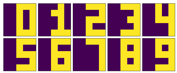
We have a set of 10 images of numbers 0..9. We want to make a neural network to predict what is the number on the image.
MODEL
Model is the term we use to refer to the network. Our model is a simple 25x10 matrix. Don't get startled by the class and the imports. It just does matrix multiplication. For now assume *model()* is a function which will take in a matrix of size (AxB) as input and mutiply it with the network weight matrix of size (BxC), to produce another matrix as output of size (AxC).
from torch import nn
import torch.nn.functional as F
import torch.optim as optim

class Model(nn.Module):
    def __init__(self):
        super(Model, self).__init__()
        self.output_layer = nn.Linear(5*5, 10, bias=False)

    def forward(self, x):
        x = self.output_layer(x)
        return F.log_softmax(x)
model = Model()
optimizer = optim.SGD(model.parameters(), lr=1, momentum=0.1)
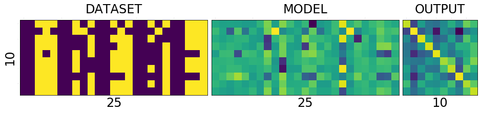
DATASET - MODEL - OUTPUT
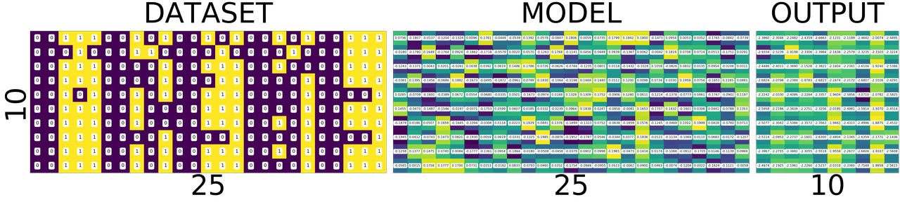
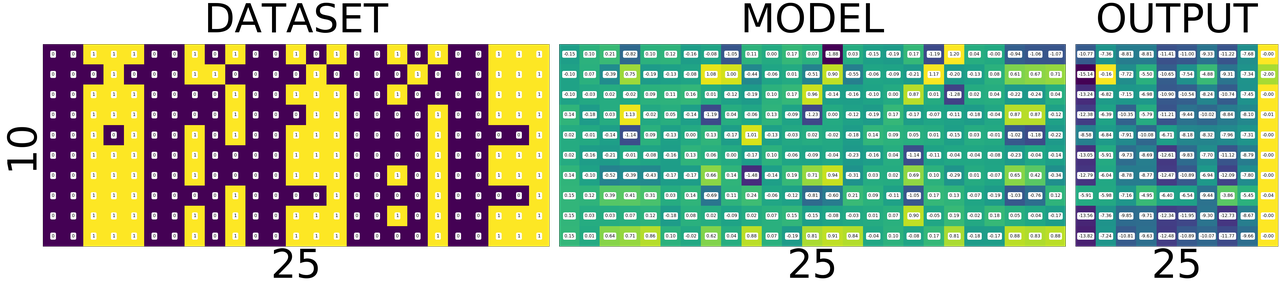
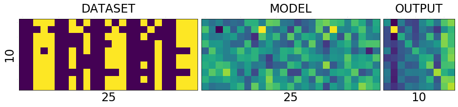
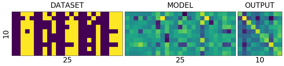
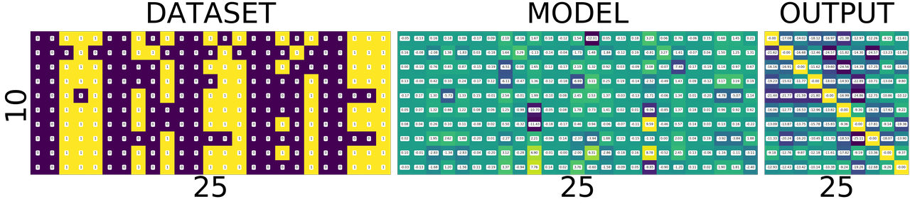
To understand the network and its training process, it is helpful to see the holy trinity INPUT-MODEL-OUTPUT
fig = plt.figure(1, (16., 16.))
grid = ImageGrid(fig, 111,
                     nrows_ncols=(1, 3),
                     axes_pad=0.1)


data = [data.view(-1) for data, target in dataset]
data = torch.stack(data)

target = [target.view(-1) for data, target in dataset]
target = torch.stack(target).squeeze()
grid[0].matshow(Image.fromarray(data.numpy()))
grid[0].set_title('DATASET', fontsize=24)
grid[0].set_ylabel('10', fontsize=24)
grid[0].set_xlabel('25', fontsize=24)
grid[0].tick_params(axis='both', which='both', length=0, labelsize=0)

grid[1].matshow(Image.fromarray(model.output_layer.weight.data.numpy()))
grid[1].set_title('MODEL', fontsize=24)
grid[1].set_xlabel('25', fontsize=24)
grid[1].tick_params(axis='both', which='both', length=0, labelsize=0)


output = model(Variable(data))
grid[2].matshow(Image.fromarray(output.data.numpy()))
grid[2].set_title('OUTPUT', fontsize=24)
grid[2].set_xlabel('10', fontsize=24)
grid[2].tick_params(axis='both', which='both', length=0, labelsize=0)

plt.show()
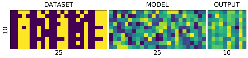
Lets try to understand what is in the picture above.
The first one is the collection of all the data that we have. The second one is the matrix of weights connecting the input of 25 input neurons to 10 output neurons. And the last one we will get to it little later.
What is special about 25 and 10 here?
Nothing. Our dataset is a set of images of numbers each having a size of 5x5 ==> 25. And we have how many different numbers a hand? 0,1,2...9 ==> 10 numbers or 10 different classes of output(this will become clear in the next post)
What is that weird picture on the left, having weird
- zero in the top-left,
- and three on the bottom-right
- and some messed up fours and eights in the middle.
Let get to it. Look the picture below.
fig = plt.figure(1,(12., 12.))
grid = ImageGrid(fig, 111,
                 nrows_ncols=(2 , 5),
                 axes_pad=0.1)

for i, (d, t) in enumerate(dataset):
    grid[i].matshow(Image.fromarray(d.numpy()))
    grid[i].tick_params(axis='both', which='both', length=0, labelsize=0)

plt.show()

fig = plt.figure(1, (100., 10.))
grid = ImageGrid(fig, 111,
                     nrows_ncols=(len(dataset), 1),
                     axes_pad=0.1)


data = [data.view(1, -1) for data, target in dataset]

for i, d in enumerate(data):
    grid[i].matshow(Image.fromarray(d.numpy()))
    grid[i].set_ylabel('{}'.format(i), fontsize=36)
    grid[i].tick_params(axis='both', which='both', length=0, labelsize=0)
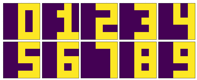
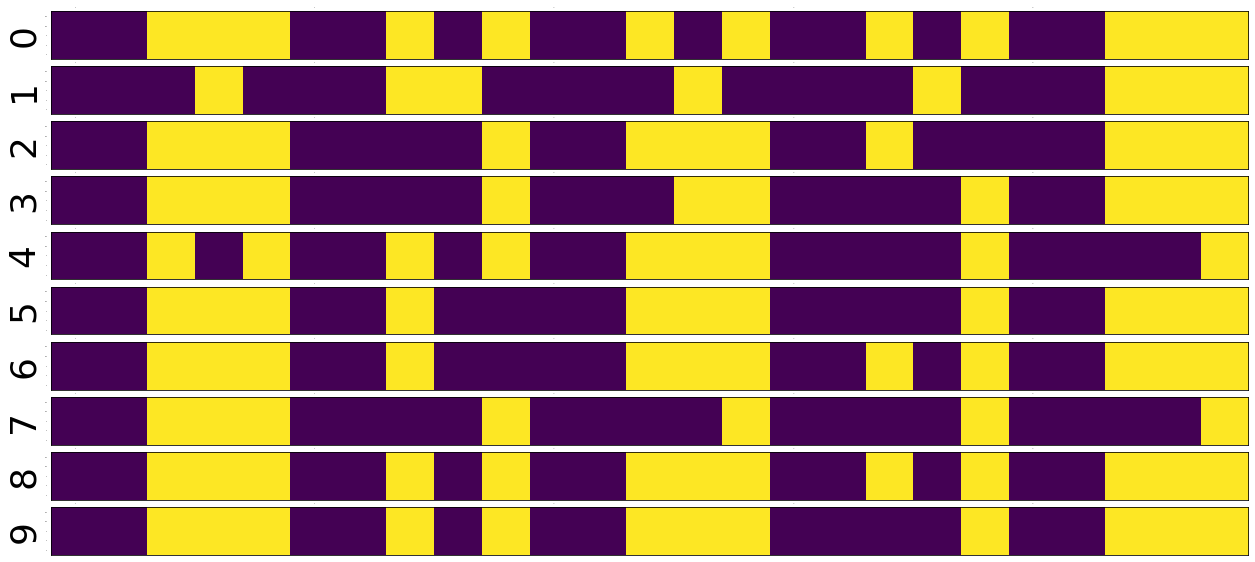
Voila!! We have just arranged the image matrix into a vector. TODO why?
This is important to remember, a simple neural network looks at the input and try to figure out which class does this input belong to
In our case inputs are the images of numbers, and outputs are how similar are the classes to the input. The output neuron with highest value is closer(very similar) to the input and the output neuron with least value is very NOT similar to the input. The inputs are real valued - it can take any numerical value but the output is discrete, a whole number corresponding to index of the neuron with largest numerical value. Also note that output of the network does not mean output of neurons.
For example after training, if we feed the image of number 3, the output neurons corresponding to 3, 8, 9 and probably 7 will have larger values and the output neurons corresponding to 1 and 6 will have the least value. Don't worry if you don't understand why, it will become clearer as we go on.
How many correct predictions without any training
Too much theory, lets get our hands dirty. Let see how many numbers did our model predicted correctly.
# Remember that output = model(Variable(data))
pred = output.data.max(1)[1].squeeze()
print(pred.size(), target.size())
correct = pred.eq(target.long()).sum()
print('correct: {}/{}'.format(correct, len(dataset)))
torch.Size([10]) torch.Size([10])
correct: 1/10
(N)ONE out of TEN
That is right it predicted none out of ten. We feeded our network with all of our data and asked it to figure what is the number that is in the image. Remember what we learned earlier about output neurons. The neural network tell us which number is present in the image by lighting up that corresponding neuron. Lets say if gave 6, the network will light up the 6th neuron will be the brightest, i.e the 6th neurons value will be the highest compared to all other neurons.
But our network above lit up wrong bulbs, for all the output. None out of ten. But why? Isn't neural network are supposed to smarter? Well yes and no. That is the difference between traditional image processing algorithms and neural networks.
Wait, let me tell you a story, that I heard. During the second world war, there were skilled flight spotter. Their job was to spot and report if any air craft was approaching. As the war got intense, there was need for more spotters and there were lot of volunteers even from schools and colleges but there was very little time to train them. So the skilled spotters, listed out a set of things to look for in the enemy flights and asked the new volunteers to memorize them as part of the training. But the volunteers never got good at spotting. Ooosh, we will continue the story later, lets get back to the point.
In classical image processing systems, we humans think, think and think and think a lot more and come up a set of rules or instructions, just like those skilled spotters. We give those instructions to the system, to make it understand how to process the images to extract information(called features - things to look for in the enemy flight) from them, and then use that information to make further decisions, such predicting what number is in the image. We feed that system with knowledge first before asking it to do anything for us.
But did we feed any knowledge to network? We just told it the input size is 25 and output size is 10. How can you expect someone to guess what is in your hand, by just telling them its size. That is rude of you. Shame on you. Okay okay. How do we make the system more knowledgable about the input? Training. The holy grail of deep learning.
What is training?
We know that the knowledge of the neural network is in the weights of the connections - represented as matrix above. We also know that by multiplying this matrix by an input image vector we will get an output which is a set of scores that describes, how similar the input is to the output neurons.
Imagine giving random values to the weights and feed the network with our data and see whether it predicts all our numbers correctly. If it did, fine and dandy, but if not give random values to the weights again and repeat the process until our network predicts all the numbers correctly. That is training in most simple form.
But think about how long will it take to find such random magical values for every weight in the network to make it work as expected. We don't know that for sure. right? You wanna continue the story. don't you? Alright.
The skilled people tried as much as they can to identify the distinguishing features of the home and enemy air crafts and tried to make the volunteers understand them. It never worked. Then they changes the strategy. They put them on the job and made them learn themselves. i.e every skilled spotter will have ten volunteers and whenever an aircraft is seen, the volunteers will shout the kind of the plane, say 'german'. Then the skilled one, will reveal the correct answer. This technique was extrememly sucessful, a spotter sent in an emergency message not only identifying it as a German aircraft, but also the correct make and model..more
Hey, why don't we try the same with our network? Lets feed the images into it and shout the answer into its tiny little output neurons so that it can update its weights by itself. Now I know you're asking how can we expect, a dumb network which cannot even predict a number in an image to train itself? Well that is where it gets interesting. We can't. Backpropgation to the rescue. It is the algorithm to update the weights of the network on our behalf.
It looks at how difference between output of network and desired output, changes with respect to the weights, and then it modifies the weights based on it. [2]
So now you understand why it predicted none out of ten correctly.
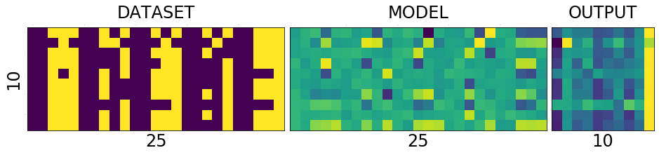
import sys
def test_and_print(model, dataset, title='', plot=True):

    data = [data.view(-1) for data, target in dataset]
    data = torch.stack(data).squeeze()

    target = [target.view(-1) for data, target in dataset]
    target = torch.stack(target).squeeze()
    output = model(Variable(data))

    loss = F.nll_loss(output, Variable(target.long()))

    dataset_img = Image.fromarray(data.numpy())
    model_img   = Image.fromarray(model.output_layer.weight.data.numpy())
    output_img  = Image.fromarray(output.data.numpy())

    pred = output.data.max(1)[1]
    correct = pred.eq(target.long()).sum()

    print('correct: {}/{}, loss:{}'.format(correct, len(dataset), loss.data[0]))
    sys.stdout.flush()

    if plot:
        fig = plt.figure(1,(16., 16.))
        grid = ImageGrid(fig, 111,
                         nrows_ncols=(1 , 3),
                         axes_pad=0.1)

        grid[0].matshow(dataset_img)
        grid[0].set_title('DATASET', fontsize=24)
        grid[0].tick_params(axis='both', which='both', length=0, labelsize=0)
        grid[0].set_ylabel('10', fontsize=24)
        grid[0].set_xlabel('25', fontsize=24)

        grid[1].matshow(model_img)
        grid[1].set_title('MODEL', fontsize=24)
        grid[1].tick_params(axis='both', which='both', length=0, labelsize=0)
        grid[1].set_xlabel('25', fontsize=24)

        grid[2].matshow(output_img)
        grid[2].set_title('OUTPUT', fontsize=24)
        grid[2].tick_params(axis='both', which='both', length=0, labelsize=0)
        grid[2].set_xlabel('10', fontsize=24)

        plt.show()


    return dataset_img, model_img, output_img
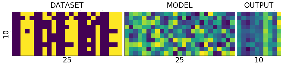
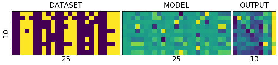
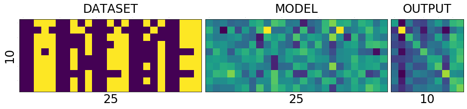
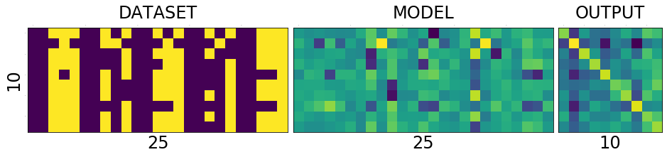
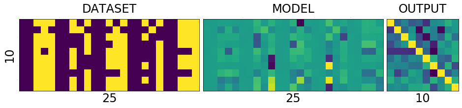
Lets take a closer look at DATASET - MODEL - OUTPUT
and understand what those colors mean.[1]
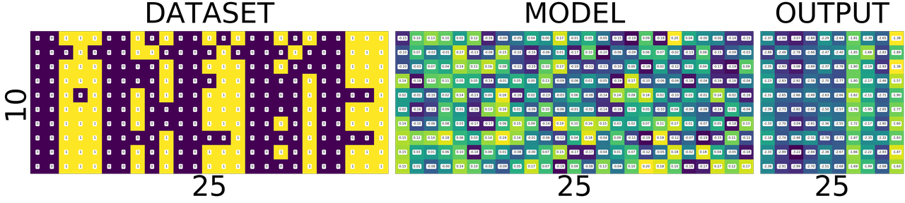
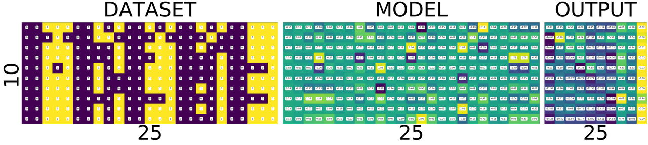
import numpy
fig = plt.figure(1, (80., 80.))
grid = ImageGrid(fig, 111,
                     nrows_ncols=(1, 3),
                     axes_pad=0.5)


data = [data.view(-1) for data, target in dataset]
data = torch.stack(data)

target = [target.view(-1) for data, target in dataset]
target = torch.stack(target)

grid[0].matshow(Image.fromarray(data.numpy()))
grid[0].set_title('DATASET', fontsize=144)
grid[0].tick_params(axis='both', which='both', length=0, labelsize=0)
grid[0].set_ylabel('10', fontsize=144)
grid[0].set_xlabel('25', fontsize=144)
for (x,y), val in numpy.ndenumerate(data.numpy()):
     grid[0].text(y, x, '{:d}'.format(int(val)), ha='center', va='center', fontsize=24,
            bbox=dict(boxstyle='round', facecolor='white', edgecolor='white'))


grid[1].matshow(Image.fromarray(model.output_layer.weight.data.numpy()))
grid[1].set_title('MODEL', fontsize=144)
grid[1].tick_params(axis='both', which='both', length=0, labelsize=0)
grid[1].set_xlabel('25', fontsize=144)
for (x,y), val in numpy.ndenumerate(model.output_layer.weight.data.numpy()):
     grid[1].text(y, x, '{:0.04f}'.format(val), ha='center', va='center',fontsize=16,
            bbox=dict(boxstyle='round', facecolor='white', edgecolor='white'))

output = model(Variable(data))
grid[2].matshow(Image.fromarray(output.data.numpy()))
grid[2].set_title('OUTPUT', fontsize=144)
grid[2].tick_params(axis='both', which='both', length=0, labelsize=0)
grid[2].set_xlabel('10', fontsize=144)

for (x,y), val in numpy.ndenumerate(output.data.numpy()):
     grid[2].text(y, x, '{:0.04f}'.format(val), ha='center', va='center',fontsize=16,
            bbox=dict(boxstyle='round', facecolor='white', edgecolor='white'))


plt.show()
If you zoom in the picture you will see numbers corresponding to the colors - violet means the lowest value, and yellow is the highest values. i.e violet does not mean 0 and yellow does not mean 1 as you might think from the dataset image.
WHAT DOES EACH ROW MEAN?
DATASET
numbers, each row is a number. first one is 0 second one is 1 and so on.
MODEL
weights corresponding to pixels in the image for a number. first row is for 0 and last one is for 9.
OUTPUT
scores of similarity. how similar the input image to all output numbers. First row contains scores of 0, how similar it is to all other numbers first square in the first row is how simlilar 0 is to 0, second square similar it is to 1. Now the scores are not only incorrect but stupid. This will become better and clear as we train the network. Lets take look at the DATASET-MODEL-OUTPUT trinity once again before training
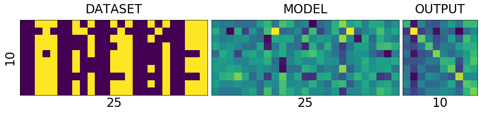
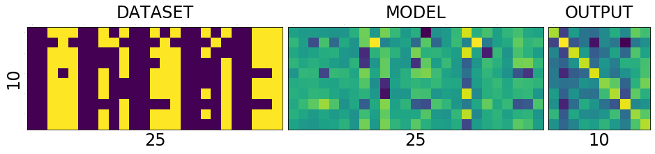
Take look at the following. It shows a single row from the output image. Go on pick the darkest square in the output above. Which row has the darkeset one?, it seems like the row corresponding to number 4, i.e data[4] the least value from that row is -3.0710
print(model(Variable(data[4].view(1, -1))))
Variable containing:
-2.2242 -2.0100 -2.4086 -2.2264 -2.3357 -1.9604 -2.5856 -3.0710 -2.0782 -2.5825
[torch.FloatTensor of size 1x10]
Similarly the brightest yellow is in the row corresonding to number 1 whose value is -1.9198 you can see below. The reason I am stressing about this fact is, this is will influence how we interpret the following images.
print(model(Variable(data[1].view(1, -1))))
Variable containing:
-2.9334 -2.5239 -1.9198 -2.3306 -2.3984 -2.1636 -2.2579 -2.3235 -2.1503 -2.3224
[torch.FloatTensor of size 1x10]
import numpy
def plot_with_values(model, dataset, title=''):
    fig = plt.figure(1, (80., 80.))
    grid = ImageGrid(fig, 111,
                         nrows_ncols=(1, 3),
                         axes_pad=0.5)


    data = [data.view(-1) for data, target in dataset]
    data = torch.stack(data)

    target = [target.view(-1) for data, target in dataset]
    target = torch.stack(target)

    plot_data = [data, model.output_layer.weight.data, model(Variable(data)).data]
    for i, tobeplotted in enumerate(plot_data):
        grid[i].matshow(Image.fromarray(tobeplotted.numpy()))
        grid[i].tick_params(axis='both', which='both', length=0, labelsize=0)
        for (x,y), val in numpy.ndenumerate(tobeplotted.numpy()):
            if i == 0: spec = '{:d}';  val = int(val)
            else: spec = '{:0.2f}'
            grid[i].text(y, x, spec.format(val), ha='center', va='center', fontsize=16,
                bbox=dict(boxstyle='round', facecolor='white', edgecolor='white'))

    grid[0].set_title('DATASET', fontsize=144)
    grid[0].set_ylabel('10', fontsize=144)
    grid[0].set_xlabel('25', fontsize=144)

    grid[1].set_title('MODEL', fontsize=144)
    grid[1].set_xlabel('25', fontsize=144)

    grid[2].set_title('OUTPUT', fontsize=144)
    grid[2].set_xlabel('25', fontsize=144)

    plt.show()
Training
Train for a single epoch
Training for a single epoch means run over all the ten images we have now.
def train(model, optim, dataset):
    model.train()
    avg_loss = 0
    for i, (data, target) in enumerate(dataset):
        data = data.view(1, -1)
        data, target = Variable(data), Variable(target.long())
        optimizer.zero_grad()
        output = model(data)

        loss = F.nll_loss(output, target)
        loss.backward()
        optimizer.step()
        avg_loss += loss.data[0]

    return avg_loss/len(dataset)
Train the model once and see how it works
train(model, optimizer, dataset)
7.596218156814575
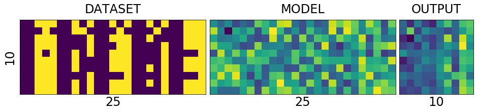
test_and_print(model, dataset)
plot_with_values(model, dataset)
correct: 2/10, loss:5.988691329956055
train once again
train(model, optimizer, dataset)
6.19214208945632
test_and_print(model, dataset)
plot_with_values(model, dataset)
correct: 2/10, loss:5.175973892211914
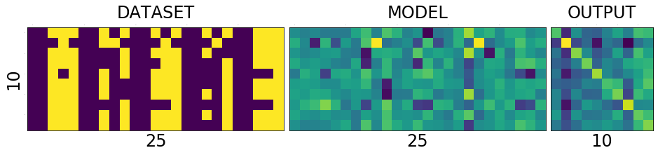
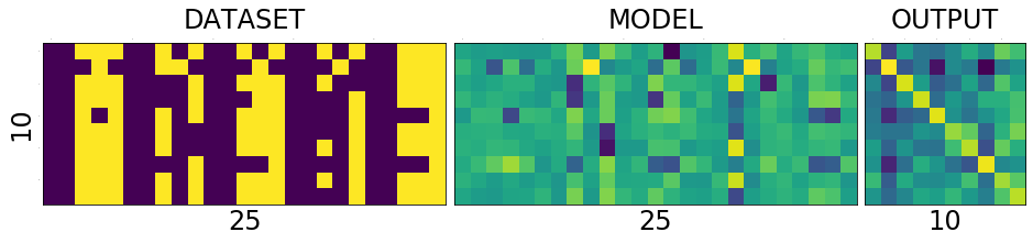
As you can see the diagonal of the output matrix is getting brighter and brighter.
That is what we want right? For each number, say for number 0. the first square in first row should be the brightest one. 1. the second square in second row should be the brightest one 2. the third square in third row should be the brightest one and so on.
Lets see the numbers directly.
Train over multiple epochs
means run over the all the samples multiple times.
def train_epochs(epochs, model, optim, dataset, print_every=10):
    snaps = []
    for epoch in range(epochs+1):
        avg_loss = train(model, optim, dataset)
        if not epoch % print_every:
            print('\n\n========================================================')
            print('epoch: {}, loss:{}'.format(epoch, avg_loss/len(dataset)/10))
            snaps.append(test_and_print(model, dataset, 'epoch:{}'.format(epoch)))

    return snaps
model = Model()
optimizer = optim.SGD(model.parameters(), lr=0.1, momentum=0.1)
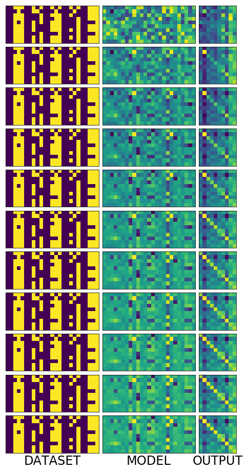
Lets train for 100 epochs and see how the model evolves. We see that in the output image, the diagonal get brigher and brighter and some other pixels getting darker and darker. It appears to be smoothing over time. Also see that after just 10 epochs the network predicts 9/10 correctly and then after 20 epochs it mastered the task, predicting 10/10 all the time. But we already know that is what we want and we know why. Lets focus on the model now, because that is where the secret lies.
snaps = train_epochs(20, model, optimizer, dataset, print_every=2)
========================================================
epoch: 0, loss:0.027155441761016846
correct: 3/10, loss:2.128438949584961
========================================================
epoch: 2, loss:0.023229331612586973
correct: 5/10, loss:1.8037703037261963
========================================================
epoch: 4, loss:0.01998117029666901
correct: 6/10, loss:1.533529281616211
========================================================
epoch: 6, loss:0.01730852520465851
correct: 8/10, loss:1.3195956945419312
========================================================
epoch: 8, loss:0.015147660285234451
correct: 9/10, loss:1.150416612625122
========================================================
epoch: 10, loss:0.013388317018747329
correct: 9/10, loss:1.0151952505111694
========================================================
epoch: 12, loss:0.011944577842950822
correct: 10/10, loss:0.9058278799057007
========================================================
epoch: 14, loss:0.010749261453747749
correct: 10/10, loss:0.8161996006965637

========================================================
epoch: 16, loss:0.009749157413840293
correct: 10/10, loss:0.7417219281196594
========================================================
epoch: 18, loss:0.008902774766087532
correct: 10/10, loss:0.6789848208427429
========================================================
epoch: 20, loss:0.008178293675184248
correct: 10/10, loss:0.6254634857177734

Lets put all those picture above into a single one to get a big picture
fig = plt.figure(1, (16., 16.))
grid = ImageGrid(fig, 111,
                     nrows_ncols=(len(snaps) , 3),
                     axes_pad=0.1)

for i, snap in enumerate(snaps):
    for j, image in enumerate(snap):
        grid[i * 3 + j].matshow(image)
        grid[i * 3 + j].tick_params(axis='both', which='both', length=0, labelsize=0)


grid[i * 3 + 0].set_xlabel('DATASET', fontsize=24)
grid[i * 3 + 1].set_xlabel('MODEL', fontsize=24)
grid[i * 3 + 2].set_xlabel('OUTPUT', fontsize=24)

plt.show()
The following animation show the state of the model over 50 epochs.
Animation
Lets train it for few thousand epochs so the network get more clear picture of the data before diving into the model :)
snaps = train_epochs(100000, model, optimizer, dataset, print_every=20000)
========================================================
epoch: 0, loss:0.007853959694504737
correct: 10/10, loss:0.60155189037323
========================================================
epoch: 20000, loss:7.162017085647676e-06
correct: 10/10, loss:0.0007155142375268042

========================================================
epoch: 40000, loss:3.5982332410640085e-06
correct: 10/10, loss:0.0003596492169890553

========================================================
epoch: 60000, loss:2.403507118287962e-06
correct: 10/10, loss:0.00024027279869187623

========================================================
epoch: 80000, loss:1.8094693423336138e-06
correct: 10/10, loss:0.00018090286175720394

========================================================
epoch: 100000, loss:1.4504563605441945e-06
correct: 10/10, loss:0.0001450170821044594
test_and_print(model, dataset)
plot_with_values(model, dataset)
correct: 10/10, loss:0.0001450170821044594

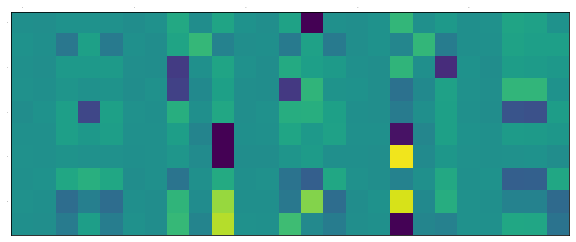
_model = model.output_layer.weight.data.numpy()
plt.figure(1, (25, 10))
plt.matshow(_model, vmin=-10, vmax = 10)
plt.tick_params(axis=u'both', which=u'both',length=0, labelsize=0)
plt.show()

fig = plt.figure(1,(10., 10.))
grid = ImageGrid(fig, 111,
                 nrows_ncols=(2 , 5),
                 axes_pad=0.1)

for i, (data, target) in enumerate(dataset):
    grid[i].matshow(Image.fromarray(data.numpy()))
    grid[i].tick_params(axis=u'both', which=u'both',length=0, labelsize=0)
    #grid[i].locator_params(axis=u'both', tight=None)

plt.show()
<matplotlib.figure.Figure at 0x7f61c7b2e470>


Dive into the model
At first look, the bright differentiating spots belongs to 5, 6 and 8, 9 pairs.
- Take 8 and 9, the last two rows, the squares at index 17 are clearly at extremes. To understand why look at the 17th pixel in images of 8 and 9. That is the only pixel distinguishing 8 and 9.
- Take 5 and 6, the same 17th pixel makes all the difference.
Now you may ask why the rows in model matrix corresponding to 8 and 9 are almost same but NOT exactly same except for that one single pixel. I will let you ponder over that point for a while.
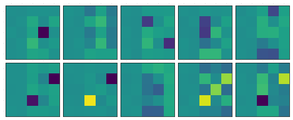
Lets reshape the model into the shape of the data. The first rows becomes the first image and second row becomes the second one...
plt.figure(1, (25, 10))
plt.matshow(_model, vmin=-10, vmax = 10)
plt.tick_params(axis=u'both', which=u'both',length=0, labelsize=0)
plt.show()

fig = plt.figure(1,(10., 10.))
grid = ImageGrid(fig, 111,
                 nrows_ncols=(2 , 5),
                 axes_pad=0.1)


for i, data in enumerate(_model):
    grid[i].matshow(Image.fromarray(data.reshape(5,5)), vmin=-10, vmax = 10)
    grid[i].tick_params(axis=u'both', which=u'both',length=0, labelsize=0)
    #grid[i].locator_params(axis=u'both', tight=None)

plt.show()
<matplotlib.figure.Figure at 0x7f61959188d0>
I don't know about you, but now I am gonna admire that picture above and wonder how beautiful neural networks are. Thank you and, ### Thanks to
- Suriyadeepan for reviewing the article
Comments